Reproducibility of a mathematical model of the neural regulation of phasic contractions and slow waves in the distal stomach
Abstract
A mathematical model of neural regulation of distal gastric interstitial cells of Cajal and smooth muscle cells was developed by Athavale et al. (2023). The model incorporated five cellular mechanisms, of which four were inhibitory and one was excitatory. The membrane potential oscillations due to phasic slow wave activity, and resulting active tension generation were simulated by the model. Neural regulation input was determined by the frequency of electrical field stimulation, and the steady-state slow wave and contraction response to this stimulation was simulated. This article appraises the reproducibility of results from Athavale et al. (2023) using the provided model analysis code. Scripts for plotting model analysis results were modified to ensure operability on Unix and Windows platforms and to ease the interpretability of figures in the absence of figure captions.
1Introduction
Neural regulation of gastric motility occurs partly through the regulation of gastric bioelectrical slow waves and phasic contractions. A mathematical model of gastric motility regulation by enteric neurons was developed to infer the relative importance of cellular mechanisms in inhibitory neural regulation of the stomach by enteric neurons and the interaction of inhibitory and excitatory stimulation.
At the cellular level, slow waves are generated and propagated by excitable pacemaker cells called interstitial cells of Cajal (ICC), which are connected in a network that exists between layers of gastric smooth muscle Sanders et al., 2006. In conjunction with excitatory and inhibitory innervation from enteric neurons, slow waves govern phasic contractions of gastric smooth muscle cells (SMC) Farrugia, 2008. These phasic contractions are responsible for the mechanical digestion and transport of food in the stomach.
2Model description
The Primary Publication describes the formulation and calibration of a model of the effects of inhibitory and excitatory enteric neural stimulation frequency ( and respectively) on self-excitatory phasic contractions of the stomach wall (Figure 1). This activity was represented by the oscillations of ICC membrane potential (), SMC membrane potential (), and active tension generation ().
Models of ICC and SMC electrophysiology were coupled by a current that was linearly proportional to the potential difference between cell membrane potential, representing the gap junction. Neural regulation was modelled by modifying equations related to the inositol triphosphate receptor (IP3R), anoctamin-1 chloride channel (Ano1), non-specific cation channel (NSCC), small conductance potassium channel (SK), and active tension components (Figure 1). The rationale for the selection of these channels and mechanisms of action is provided in the Primary Publication. Parameters for each of these pathways (, , , , and ) were calibrated to experimental data from literature Kim et al., 2003Forrest et al., 2006.
The mathematical model is self-excitatory and varying the neural regulation input altered the nature of slow wave events. The Primary Publication Athavale et al., 2023 presented algorithms to identify simulated slow wave events and calculate their frequency and plateau amplitude.
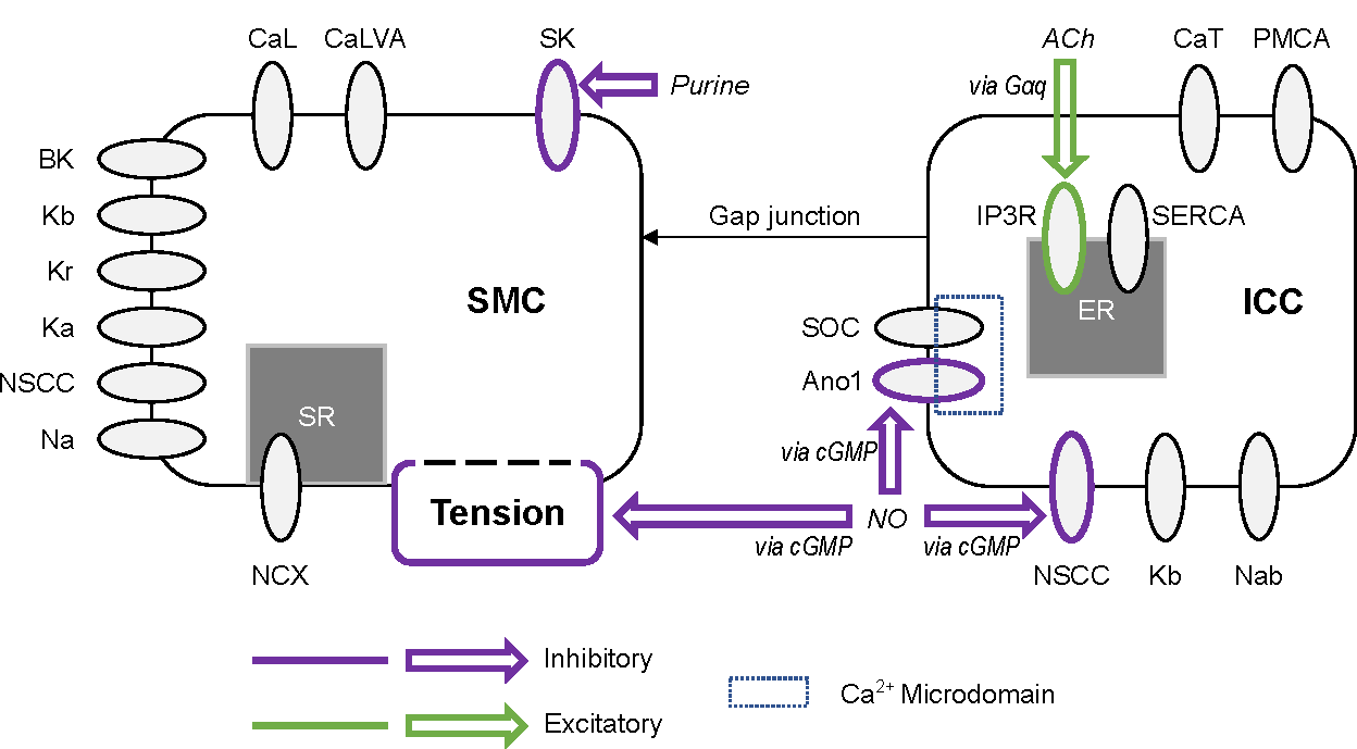
Figure 1:Outline of the coupled electrophysiology and neural regulation model of a distal gastric interstitial cell of Cajal (ICC) and gastric smooth muscle cell (SMC). Inhibitory effector components are outlined in purple and excitatory effector components are outlined in green. CaL: L-type calcium channel, CaLVA: T-type calcium channel (see also CaT in the ICC model), SK: small conductance potassium channel, BK: large conductance potassium channel, Kb: lumped background potassium current, Kr: delayed rectifying potassium channel, Ka: A-type voltage-gated potassium channel, NSCC: non-specific cationic conductance, Na: lumped sodium current, NCX: sodium-calcium exchanger, SR: sarcoplasmic reticulum, Gαq: G-protein α subunit, ACh: acetylcholine, CaT: T-type calcium channel (see also CaLVA in the SMC model), PMCA: plasma membrane calcium ATPase, IP3R: IP3-activated calcium channel, SERCA: sarcoendoplasmic reticulum calcium ATPase, SOC: store-operated calcium channel, Ano1: anoctamin-1 voltage-gated, calcium activated chloride channel, cGMP: cyclic guanosine monophosphate second messenger nucleotide, NO: nitric oxide, Nab: lumped background sodium current. This figure is reproduced with modification from Athavale et al. (2023) under a Creative Commons CC-BY 4.0 licence.
3Computational simulation
The CellML model and MATLAB model analysis code were obtained from a FigShare repository (www.doi.org/10.6084/m9.figshare.23624622.v2). The implementation of the models used to produce the figures in this article can be found at
https://github.com/OmkarAthavale/ICC_SMC_Neuro/tree/b83bd0.
The mathematical model was specified in the ICC_SMC_Neuro.cellml file. A MATLAB implementation of this model, generated through OpenCOR v0.6 Garny & Hunter, 2015, was also provided with modifications that enable parameter sweeps implemented in the model analysis scripts. A second mathematical model file, ICC_SMC_Neuro_Tvar.cellml specified the mathematical model with additional input parameters to set stimulation start and stop times. A MATLAB implementation generated using OpenCOR was also provided.
A collection of analysis scripts and helper functions were provided to generate the results reported in the Primary Publication. The reproducibility of results from the Primary Publication was assessed by running these analysis files in MATLAB 2024b (The MathWorks Inc., Natick, MA, USA) to reproduce plots from the Primary Publication. The code saved figures as scalable vector graphics (SVG) files. Using Inkscape (v1.2, InkScape Project) these were converted to PDF files (300 dpi) and are presented in this article without further modification.
4Reproducibility goals
The aim of this article is to reproduce the results shown in Figure 2, Figure 3, and Figure 5 of the Primary Publication.
5Model results
The following show the output from the model analysis code provided in the Primary Publication. Two modifications were needed to make the provided analysis scripts run successfully.
A new directory, named “generated_fig”, needed to be created prior to running model analysis scripts so that figure files were saved.
Second, the code that reads parameter sweep data (Lines 51 – 55 of figure_generation/parameter_sweep_1D_combined_plot.m) did not work on Unix platforms. This was fixed by replacing these lines with the following code snippet to allow the script to work on both Windows and Unix platforms:
if ispc
    files = ls('../data/Multi_1DSweep_*');
    nF = size(files, 1);
    for i = 1:nF
        d{i} = load(['../data/', files(i, :)]);
    end
else
    files = splitlines(ls('../data/Multi_1DSweep_*'));
    nF = size(files, 1)-1;
    for i = 1:nF
        d{i} = load([files{i}]);
    end
end
Additional changes were made to make the generated output for Figure 6 and Figure 7 more interpretable by varying line colours and adding a legend. Finally, the units for tension as labelled in the code (mN) were inconsistent with the units described by the model specification and Primary Publication (kPa) in one of the plotting scripts (figure_generation/aligned_event_plot.m). Figures 3 – 5 show the output with the correct units labelled.
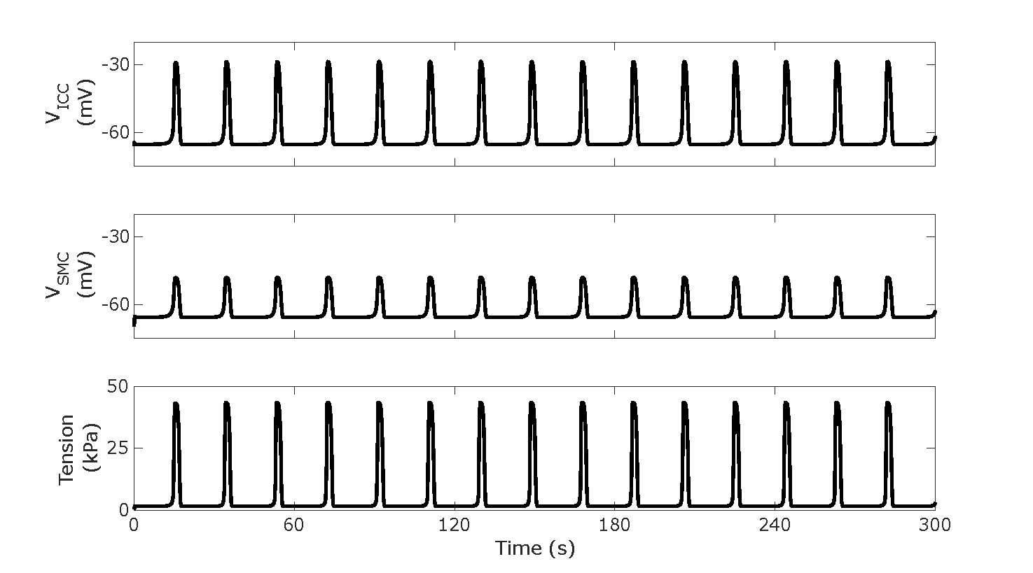
Figure 2:Slow wave and phasic contractions without any neural regulation input as shown by traces of , ), and . Reproduces Figure 2A from the Primary Publication.
Script: figure_generation/baseline_plotter.m;
Figure: generated_fig/baseline_3min_<timestamp>.svg
![A single slow wave for a sweep of parameter k_{iAno1} with values of 0.0, 0.25, 0.5, 0.75, and 1.0 with f_i set to 10 Hz. Reproduces Figure 2B Panel k_{iAno1} from the Primary Publication with the tension units corrected. Line 11 of figure_generation/aligned_event_plot.m was changed to “effect_var = [1];”. Script: figure_generation/aligned_event_plot.m; Figure: generated_fig/events_sweep_k_iAno1_<timestamp>.svg](https://pub.curvenote.com/0194f705-5e90-7bf1-a132-e53ae140ba37/public/event_sweep_Ano1-6b1047acce1ee9b949859fdc6cbac4d0.png)
Figure 3:A single slow wave for a sweep of parameter with values of 0.0, 0.25, 0.5, 0.75, and 1.0 with set to 10 Hz. Reproduces Figure 2B Panel from the Primary Publication with the tension units corrected. Line 11 of figure_generation/aligned_event_plot.m was changed to “effect_var = [1];”.
Script: figure_generation/aligned_event_plot.m;
Figure: generated_fig/events_sweep_k_iAno1_<timestamp>.svg
![A single slow wave for a sweep of parameter k_{iNSCC} with values of 0.0, 0.25, 0.5, 0.75, and 1.0 with f_i set to 10 Hz. Reproduces Figure 2B Panel k_{iNSCC} from the Primary Publication with the tension units corrected. Line 11 of figure_generation/aligned_event_plot.m was changed to “effect_var = [2];”. Script: figure_generation/aligned_event_plot.m; Figure: generated_fig/events_sweep_k_iNSCC_<timestamp>.svg](https://pub.curvenote.com/0194f705-5e90-7bf1-a132-e53ae140ba37/public/event_sweep_NSCC-bf69376a10992cb67841c9b81acada31.png)
Figure 4:A single slow wave for a sweep of parameter with values of 0.0, 0.25, 0.5, 0.75, and 1.0 with set to 10 Hz. Reproduces Figure 2B Panel from the Primary Publication with the tension units corrected. Line 11 of figure_generation/aligned_event_plot.m was changed to “effect_var = [2];”.
Script: figure_generation/aligned_event_plot.m;
Figure: generated_fig/events_sweep_k_iNSCC_<timestamp>.svg
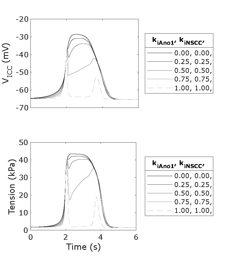
Figure 5:A single slow wave for a sweep of parameters and with both having a value of 0.0, 0.25, 0.5, 0.75, and 1.0, and with set to 10 Hz. Reproduces Figure 2B Panel & Panel from the Primary Publication with the tension units corrected. Line 11 of figure_generation/aligned_event_plot.m was unchanged.
Script: figure_generation/aligned_event_plot.m;
Figure: generated_fig/events_sweep_k_iAno1_k_iNSCC_<timestamp>.svg
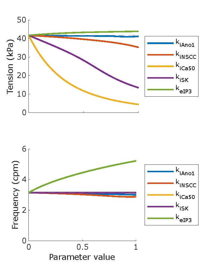
Figure 6:Phasic contraction maximum tension and frequency for sweeps of parameter values from 0 – 1 with an increment of 0.1. The non-varying parameters were set to 0. and were set to 10 Hz, and non-linear scaling terms , and were set to 1.0. Reproduces Figure 3 from the Primary Publication. Minor changes were required to correctly load the parameter sweep results for plotting, see Section 5.
Script: figure_generation/parameter_sweep_1D_combined_plot.m;
Figure: generated_fig/stimulation_varying_<timestamp>.svg
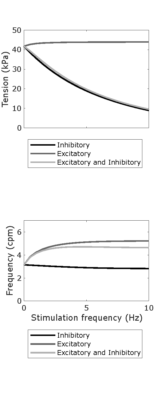
Figure 7:Parameter sweeps showing the phasic contraction amplitude and frequency across neural regulation input values for and separately from 0 – 10 Hz with an increment of 0.05 Hz. The parameter values were set to the optimised values as determined in the Primary Publication. Reproduces Figure 5A and Figure 5B from the Primary Publication.
Script: figure_generation/dosage_sweep_plot.m;
Figure: generated_fig/dosage_sweep_21_<timestamp>.svg
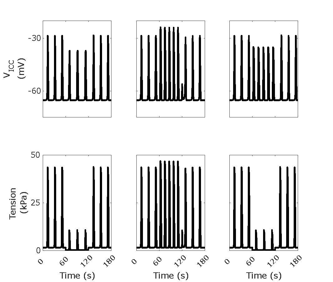
Figure 8:Traces of and for a stimulation scheme having 60 s no stimulation, then 60 s stimulation, then 60 s no stimulation. For columns from left to right, the applied stimulation is inhibitory only ( = 10 Hz), excitatory only ( = 10 Hz), and inhibitory and excitatory together( = = 10 Hz). Reproduces Figure 5C from the Primary Publication.
Script: figure_generation/stimulation_plotter.m;
Figure: generated_fig/stimulation_varying_<timestamp>.svg
6Discussion
The published model analysis files were able to reproduce results from the Primary Publication though minor inconsistencies in unit labelling and errors with data loading needed rectification. A directory was created so that figures could be saved using the model analysis script. Changes were made to figure_generation/parameter_sweep_1D_combined_plot.m to ensure that saved data were loaded without errors.
Some of the labels and colouring of plots in the Primary Publication were not reproduced by the analysis scripts. Instead alternative colouring and labelling was applied so that outputs from the plotting scripts were interpretable directly form the script output, in the absence of a figure caption.
- Athavale, O. N., Avci, R., Clark, A. R., Di Natale, M. R., Wang, X., Furness, J. B., Liu, Z., Cheng, L. K., & Du, P. (2023). Neural regulation of slow waves and phasic contractions in the distal stomach: a mathematical model. Journal of Neural Engineering, 20(6). 10.1088/1741-2552/ad1610
- Sanders, K. M., Koh, S. D., & Ward, S. M. (2006). Interstitial cells of Cajal as pacemakers in the gastrointestinal tract. Annual Reviews Physiology, 68(18), 307–343. 10.1146/annurev.physiol.68.040504.094718
- Farrugia, G. (2008). Interstitial cells of Cajal in health and disease. Neurogastroenterology and Motility, 20, 54–63. 10.1111/j.1365-2982.2008.01109.x
- Kim, T., La, J., Lee, J., & Yang, I. (2003). Effects of nitric oxide on slow waves and spontaneous contraction of guinea pig gastric antral circular muscle. J. Pharmacol. Sci., 92(4), 337–347. 10.1254/jphs.92.337
- Forrest, A. S., Ördög, T., & Sanders, K. M. (2006). Neural regulation of slow-wave frequency in the murine gastric antrum. Am. J. Physiol. - Gastrointest. Liver Physiol., 290(3), G486–G495. 10.1152/ajpgi.00349.2005
- Garny, A., & Hunter, P. J. (2015). OpenCOR: A modular and interoperable approach to computational biology. Front. Physiol., 6. 10.3389/fphys.2015.00026