Energy-based bond graph models of glucose transport with SLC transporters
Abstract
In Hunter et al. (2025), we proposed an energy-based modelling framework and presented two exemplar bond graph templates for solute carrier (SLC) transporter families: facilitated diffusion with SLC2A2 (GLUT2) and sodium-glucose cotransport with SLC5A1 (SGLT1). In this article, we provide detailed information on the parameterisation process for these two SLC families and the information required to reproduce the results presented in Hunter et al. (2025).
1Introduction
We presented the bond graph BG models for the solute carrier (SLC) family members SLC2A2 and SLC5A1 in Hunter et al. (2025). The models have been implemented using CellML Cuellar et al., 2003 and the model implementation is available in the Physiome Model Repository (PMR) Yu et al., 2011 at: https://Facilitated transporter and Electrogenic cotransporter hold the models of SLC2A2 and SLC5A1, respectively. Brief descriptions of the CellML model files can be found in the PMR exposure: https://
2Model and simulation setup
In addition to the CellML models, this study makes use of Python scripts to facilitate simulation and presentation. All files required to reproduce and reuse this study can be obtained by downloading the associated OMEX archive. Alternatively, readers familiar with git may clone the repository at https://git clone --recurse-submodules or follow the appropriate instructions based on your Git client.
After obtaining the required files, a Python environment with the required capabilities can be created by installing the dependencies listed in the requirements.txt file. This can be done using a command similar to pip install -r requirements.txt or by following the appropriate procedure for the chosen platform.
The src folder contains Python scripts for running simulations, processing simulation results, and plotting data. The primary scripts relevant to this manuscript are summarised here as well as mentioned as they are used in the following sections.
sim_GLUT2.py: Performs simulations of SLC2A2 and saves the results to </Facilitated transporter/CellMLV2/sim_results>.sim_SGLT1.py: Performs simulations of SLC5A1 and saves the results to </Electrogenic cotransporter/CellMLV2/sim_results>.mergeData_GLUT2.py: Prepares the data in </Facilitated transporter/CellMLV2/sim_results> for plotting.mergeData_SGLT1.py: Prepares the data in </Electrogenic cotransporter/CellMLV2/sim_results> for plotting.plot_GLUT2.py: Plots the simulation results for SLC2A2.plot_SGLT1.py: Plots the simulation results for SLC5A1.
Other Python scripts were used to generate the SED-ML files in </Facilitated transporter/CellMLV2/> and </Electrogenic cotransporter/CellMLV2/>. These SED-ML files are provided so users do not need to run the scripts again.
3SLC2A2 bond graph model parameterisation
The SLC2A2 (protein name GLUT2) uses the extracellular to intracellular glucose concentration gradient to drive transmembrane transport of glucose in a process called ‘facilitated diffusion’, and we replicated the bond graph diagram in Figure 1 for convenience. The kinetic data that we used to obtain the parameters of the bond graph model were from Lowe & Walmsley (1986), and the kinetic model diagram is shown in Figure 2. Note that the notation and the parameter names in the kinetic diagram are different from the bond graph. Additionally, the bond graph model of SLC2A2 can be generalised and parameterised to represent any member of the SLC2 family. The data from Lowe & Walmsley (1986) were measured for SLC2A1/GLUT1, while SLC2A2/GLUT2 is used in this Physiome paper to remain consistent with the primary reference Hunter et al. (2025).
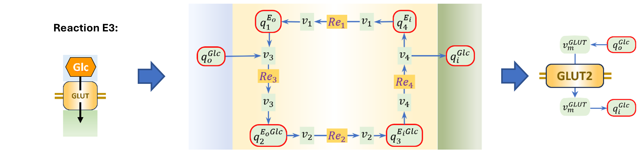
Figure 1:Bond graph of SLC2A2, replicated from Hunter et al. (2025).
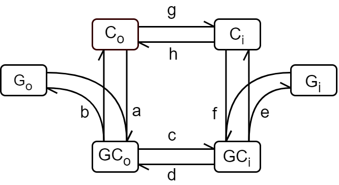
Figure 2:Kinetic model diagram adapted from Lowe & Walmsley (1986). Note that the notations for the conformation states of the transporter are different from the bond graph: ; ; ; ; ; . The letters associated with the edges are the rate constants and the arrows indicate the flux directions.
Table 1 lists the kinetic parameters, which are the rate constants associated with the forward and reverse reaction fluxes in the traditional mass-action equations. The first column of Table 1 is the corresponding parameter names for the reactions in the bond graph where the subscript indicates the reaction number, while the second column lists the kinetic parameter names in Lowe & Walmsley (1986).
Table 1:The kinetic parameters in Lowe & Walmsley (1986).
| Kinetic in BG | Parameter in Lowe & Walmsley (1986) | Value | Unit |
| 0.726 | |||
| 1113 | |||
| 4.5e7[1] | |||
| [2] | |||
| 12.1 | |||
| 90.3 | |||
| [3] | |||
| 2.7e5[1] |
3.1Bond graph parameters
Pan (2019) introduced a method to convert kinetic parameters to bond graph parameters provided that the kinetic models are thermodynamically consistent. Here, we use the SLC2A2 example to detail the link between the kinetic parameters in traditional mass-action equations and bond graph parameters. In particular, kinetic models often capture the fluxes using the unit such as , while bond graph usually explicitly models the flow rate using the unit such as and potentials using the unit for biochemical reactions. When we convert the kinetic parameters to bond graph parameters, we need to consider such dimensional differences.
Conventionally, the rate of biochemical reactions can be described by the law of mass action. The rate of the forward reaction () (also known as forward flux) is proportional to the amount of the reactants (E, as shown in Equation 1), while the rate of the reverse reaction () (also known as reverse flux) is proportional to the amount of the products (P, as shown in Equation 2). () and () are the concentrations of reactants and products, and are the forward and reverse rate constants, while and are the corresponding stoichiometric coefficients.
The total rate of reaction () (i.e., net flux) is expressed in Equation 3.
In the case of the reaction network of SLC2A2 (Figure 1), we can express the fluxes using Equation 4.
The bond graph formulation highlights thermodynamic consistency and the flow of chemical species is driven by the chemical potentials Pan, 2019. The chemical potential of a specicies is determined by the molar amount of (), shown in Equation 5, where () is the ideal gas constant, () is the absolute temperature and () is the thermodynamic constant of the species.
The rate of a reaction () can be expressed using the Marcelin-de Donder equation (Equation 6). () is the forward affinity (the total chemical potential of the reactants) and () is the reverse affinity (the total chemical potential of the products).
For example, the flow rate of the reaction in Figure 1 can be given by Equations 7, 8 and 9.
Equation 7 can be rearranged as Equation 10 by substituting Equations 8 and 9 into Equations 7.
The flow rates of the reaction network of SLC2A2 (Figure 1), can be expressed using Equation 11.
The relationship between the molar amount () and the concentration () of a species is , where () is the volume of the compartment in which the species resides. Equation 11 can be rewritten as Equation 12 if we incorporate the concentrations of species rather than the molar amount.
By comparing Equations 4 and 12, we can see the relationship between the kinetic parameters (, ) and the bond graph parameters (, ):
By defining as an element-wise logarithm operator, Equation 13 can be linearized and rewritten as the matrix equation:
In Pan (2019), the above equation was generalised using Equation 15.
where
is an identity matrix of length , while is the number of reactions. and are the transpose of forward and reverse stoichiometric matrices and , respectively. The vectors of the forward and reverse kinetic rate constants , , and the vector of known constraints between the species defined in the matrix for SLC2A2 are shown in Equation 17.
The orders of the elements in and are the same order of the reactions, organized as columns in the matrices and , shown in Table 2 and Table 3, while is organized by [number of species][number of ]. Note that we do not need to add constraints in this case therefore both and are empty.
Table 2:Forward stoichiometric matrix for the SLC2A2.
[head=false, tabular=ccccc, table head=, late after line=
, late after first line=
, table foot=, ]SLC2_f_Copy.csv & & & &
Table 3:Reverse stoichiometric matrix for the SLC2A2.
[head=false, tabular=ccccc, table head=, late after line=
, late after first line=
, table foot=, ]SLC2_r_Copy.csv & & & &
The diagonal matrix (Equation 18) accounts for the volumes of compartments and the size is 10 ([number of reactions][number of species]). The typical blood cell volume () according to McLaren et al. (1987) and we set the extracellular volume () as well. Since the protein SLC2A2 does not exist in a compartment, we set volumes of corresponding conformations of the protein () Pan, 2019. That is, their thermodynamic constants are not related to the volumes.
Given the above vectors and matrices, we can obtain bond graph parameters by matrix inversion (Equation 19),
where is the Moore-Penrose pseudoinverse of and is the element-wise exponential. The resulting bond graph parameters based on Equation 19 are shown in Table 4.
Table 4:The bond graph parameters of the full BG model for SLC2A2.
[head=false, tabular=ccc, table head=, late after line=
, late after first line=
, table foot=, ]SLC2_BG.csv & &
3.2Parameters for steady state
Hunter et al. (2025) provided the analytical expression in Equation 20 Hunter et al., 2025 to calculate the parameters for the steady-state flux in Equation 19 Hunter et al., 2025 using the bond graph parameters in Table 4. We refer the readers to the primary paper for the analytical derivation process and calculation, while we explain here how we obtained the parameters from the steady-state data Lowe & Walmsley, 1986.
The Michaelis-Menten formulation of zero trans influx Lowe & Walmsley, 1986 of the transporter, i.e., set the intracellular concentration to be 0 (), is shown in Equation 20,
where is the extracellular concentration of glucose, the maximum flux is calculated using Equation 21 with the concentration of glucose carrier molecules in human red blood cells of 6.67 () Lowe & Walmsley, 1986.
The Michaelis-Menten constant of Equation 20 is calculated using Equation 22 Lowe & Walmsley, 1986, where is the dissociation constant of reaction .
When the intracellular molar amount of glucose is zero, the steady-state expression (Equation 19 in Hunter et al. (2025)) can be rearranged to Equation 23.
Substitute in the above equation with , and add the () term to convert the unit from to and rearrange it to Equation 24.
We obtain the following relationships in Equations 25 and 21 by comparing Equations 20 and 24.
Hence, we obtained the parameters and using Equations 27 and 28.
The Michaelis-Menten of zero trans efflux Lowe & Walmsley, 1986 i.e., set the extracellular concentration to be 0 (), is shown in Equation 29.
, where is the intracellular concentration of glucose, and the maximum flux is calculated using Equation 30 Lowe & Walmsley, 1986.
The Michaelis-Menten constant is calculated using Equation 31 Lowe & Walmsley, 1986, where is the dissociation constant of reaction .
When the extracellular molar amount of glucose is zero, the steady-state expression (Equation 19 in Hunter et al. (2025)) can be rearranged to Equation 32.
Substitute in the above equation with , and add the () term to convert the unit from to and rearrange it to Equation 33.
By comparing Equations 29 and 33, we obtained Equation 34.
Then we can calculate the parameter using Equation 35.
is calculated using Equation 20 in Hunter et al. (2025). The parameters are summarized in Table 5.
Table 5:The parameters of the steady state bond graph model for SLC2A2.
| Parameter | Value | Unit |
| 0.003284 | ||
| 1.4735 | dimensionless | |
| 21.671 | dimensionless | |
| 235.07 | dimensionless |
3.3Simulation results
We encoded the full bond graph model Hunter et al., 2025 in GLUT2_BG.cellml and the parameters in params_BG.cellml. To simulate the inward flux, we set the molar amount of intracellular glucose to be a very small value (), and varied the molar amount of extracellular glucose from () to 2.25 (). For each extracellular glucose value, we simulate the model for 250 seconds to get the steady-state flow rate. Similarly to simulate the outward flux, we set the molar amount of extracellular glucose to be a very small value (), and varied the molar amount of intracellular glucose from () to 2.25 (). For each intracellular glucose value, we simulate the model for 250 seconds to get the steady-state flow rate.
We encoded the Equations 20 and 29 in GLUT2_kinetic.cellml and simulated the zero trans influx and efflux by varying the extracellular glucose concentration and intracellular glucose concentration respectively from () to 25 ().
The steady-state model in Equations 19 and 20 in Hunter et al. (2025) were encoded in
GLUT2_ss_oi.cellml and GLUT2_ss_io.cellml. GLUT2_ss_oi.cellml sets the molar amount of intracellular glucose to be very small value () and varies the molar amount of extracellular glucose from () to 2.25 (); GLUT2_ss_io.cellml sets the molar amount of extracellular glucose to be very small value () and varies the molar amount of intracellular glucose from () to 2.25 ().
Figure 3 shows the steady-state fluxes from the full bond graph model and steady-state model in Hunter et al. (2025) compared to the zero trans influx (Equation 20) and efflux (Equation 29) in Lowe & Walmsley (1986). The plots in red used the parameters in Table 5 for Equation 19 in Hunter et al. (2025), while the magenta lines used the parameters in Table 4 to calculate the parameters for Equation 19 in Hunter et al. (2025) according to Equation 20 in Hunter et al. (2025).
![(a) Inward flux as a function of [A]_o when [A]_i =0, and (b) outward flux as a function of of [A]_i when [A]_o =0. Note that in order to compare with the kinetic data in , the molar amount of glucose in the bond graph model was converted to glucose concentrations.This is Figure 8 in .](https://pub.curvenote.com/019992e3-2ea5-72a7-85c1-3c73ef224b6b/public/GLUT2_fit_ss_new-7cc6a07b4aa7f79988110dae5be99754.png)
Figure 3:(a) Inward flux as a function of when , and (b) outward flux as a function of of when . Note that in order to compare with the kinetic data in Lowe & Walmsley (1986), the molar amount of glucose in the bond graph model was converted to glucose concentrations.This is Figure 8 in Hunter et al. (2025).
We summarize the models, parameters, and corresponding simulation plots in Table 6. We have provided the Python scripts under the folder <src> to run the simulations and plot the data, while the SED-ML files in <Facilitated transporter\ CellMLV2> detail the simulation settings. To get the result in Figure 3, the Python scripts sim_GLUT2.py, mergeData_GLUT2.py, plot_GLUT2.py should run in sequence.
Table 6:Summary of the model files, parameters and corresponding simulation plots in Figure 3
| Model file | Parameters | Plot in Figure 3 |
| GLUT2_kinetic.cellml | Table 1 | Lowe AG and Walmsley AR (1986) in Figure 3 (a) and (b) |
| GLUT2_BG.cellml | Table 4 | Bond graph in Figure 3 (a) and (b) |
| GLUT2_ss_oi.cellml | Table 4 for Steady-state Eqs 19 and 20 and Table 5 for Steady-state Eq. 19 | Steady-state Eq. 19 and Steady-state Eqs 19 and 20 in Figure 3 (a) |
| GLUT2_ss_io.cellml | Table 4 for Steady-state Eqs 19 and 20 and Table 5 for Steady-state Eq. 19 | Steady-state Eq. 19 and Steady-state Eqs 19 and 20 in Figure 3 (b) |
4SLC5A1 bond graph model parameterization
The SLC5A1 (SGLT1) uses the sodium gradient to drive glucose into the cell, typically when the transmembrane glucose gradient is insufficient to provide the required flux of glucose. The bond graph is shown in Figure 4. We parameterize the bond graph model to fit the data in Parent et al. (1992), and the kinetic model diagram is shown in Figure 5. Note that the notation and the parameter names in the kinetic diagram are different from the bond graph.
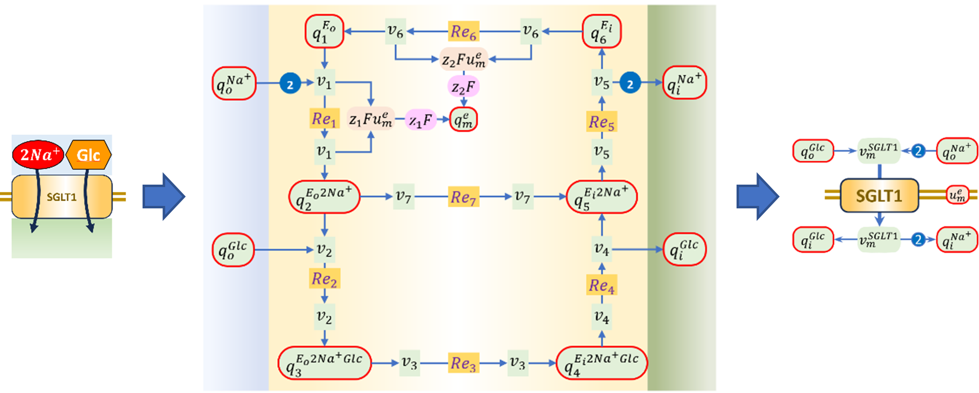
Figure 4:Bond graph of SLC5A1, replicated from Hunter et al. (2025).
![Kinetic model diagram adapted from Figure 1 of . Note that the notations are different from the bond graph: [C]^\prime-~E_o(BG); [C]^{\prime\prime}-~E_i(BG); [CNa_2]^\prime-~E_o2Na^+(BG); [CNa_2]^{\prime\prime}-~E_i2Na^+(BG); [SCNa_2]^\prime-~E_o2Na^+Glc(BG); [SCNa_2]^{\prime\prime}-~E_i2Na^+Glc(BG); [Na]^\prime-~Na_o(BG); [Na]^{\prime\prime}-~Na_i(BG);[S]^\prime-~Glc_o(BG); [S]^{\prime\prime}-~Glc_i(BG). \delta=0.7 ,\alpha^\prime=0.3 and we omitted the electrical field between [C]^{\prime\prime} and [CNa_2]^{\prime\prime} because \alpha^{\prime\prime}=0 in . \mu=\frac{FV}{RT} where V is the membrane potential, F=96485 C/mol and R=8.314J/mol/K are Faraday constant and universal gas constant, respectively, and T=293K is temperature. The letters associated with the edges are the rate constants and the arrows indicate the flux directions.](https://pub.curvenote.com/019992e3-2ea5-72a7-85c1-3c73ef224b6b/public/SLC5-7e7bf5ca8bfad20bb05f2eb87cbf9b8f.png)
Figure 5:Kinetic model diagram adapted from Figure 1 of Parent et al. (1992). Note that the notations are different from the bond graph: ; ; ; ; ; ; ; ;; . , and we omitted the electrical field between and because in Parent et al. (1992). where is the membrane potential, and are Faraday constant and universal gas constant, respectively, and is temperature. The letters associated with the edges are the rate constants and the arrows indicate the flux directions.
The kinetic parameters in in Parent et al. (1992) are listed in Table 7 and Table 8. The first column is the corresponding kinetic parameters for the reactions in the bond graph where the subscript is the reaction number. The original units in Parent et al. (1992) were , or , while the units were changed to , or in Eskandari et al. (2005) where the model Parent et al., 1992 was reused. We found that using the units in Eskandari et al. (2005) gave the right dynamic outputs, so we used , or in this article and the primary paper Hunter et al., 2025.
Table 7:The kinetic parameters for simulation of Fig. 10 in Parent et al. (1992).
| c|c|c|c|X Kinetic in BG | Parameter | Value | Unit | Remark |
| 80000 | () | |||
| 1e5 | () | |||
| 50 | ||||
| 800 | ||||
| 10 | ||||
| 5 | ||||
| 0.3 | ||||
| 500 | ||||
| 20 | ||||
| 50 | ||||
| 1.8285e7 [4] | () | |||
| 50 | () | |||
| 35 | ||||
| 1.371 [5] |
Table 8:The kinetic parameters for simulation of Fig. 5 in Parent et al. (1992).
| c|c|c|c|X Kinetic in BG | Parameter | Value | Unit | Remark |
| 80000 | () | |||
| 1e5 | () | |||
| 50 | ||||
| 800 | ||||
| 10 | ||||
| 3 | ||||
| 0.3 | ||||
| 500 | ||||
| 20 | ||||
| 50 | ||||
| 1.0971e7 [6] | () | |||
| 50 | () | |||
| 35 | ||||
| 0.823 [7] |
4.1Bond graph parameters
We apply the same method Pan, 2019 to convert the kinetic parameters to bond graph parameters. Since we have described how to link kinetic parameters to bond graph parameters in Section 3.1, we directly solve Equation 15 to get the bond graph parameters for SLC5A1 without repeating the derivation process. First, we construct matrices , , , and to get Equation 15 for SLC5A1. The vectors of the forward and reverse kinetic rate constants , are defined below and the values are from Table 7 and Table 8.
Note that we do not need to add constraints therefore both and are empty in this case. The forward and reverse stoichiometric matrices () are shown in Table 9 and Table 10, respectively. The first row lists the reactions while the first column denotes the species.
Table 9:Forward stoichiometric matrix for the SLC5A1.
[head=false, tabular=cccccccc, table head=, late after line=
, late after first line=
, table foot=, ]SLC5_f_Copy.csv & & & & & & &
Table 10:Reverse stoichiometric matrix for the SLC5A1.
[head=false, tabular=cccccccc, table head=, late after line=
, late after first line=
, table foot=, ]SLC5_r_Copy.csv & & & & & & &
Based on McLaren et al. (1987) we set the volume of blood cells to () and use the same value for the extracellular volume. The diagonal matrix that accounts for the volumes of compartments is constructed in Equation 37.
Note that when preparing this Physiome manuscript we discovered a unit conversion error of the cell volume used to calculate parameter values in the Primary paper Hunter et al., 2025. This error scaled up the thermodynamical parameters of and by 107, i.e., , and with corrected values given in Tables 11, 12 and 13. Since the product of the thermodynamical parameter and cell volume, e.g., , determines the dynamics of the system, the scaling effect () is canceled. Therefore, this change does not affect the model dynamics or simulation results.
Given that we have constructed all the matrices needed in Equation 15, we now apply the method in Equation 19 to obtain the bond graph parameters for SLC5A1, which are shown in Table 11 and Table 12.
Table 11:The bond graph parameters of the full BG model for SLC5A1 corresponding to Fig.10 of Parent et al. (1992).
[head=false, tabular=ccc, table head=, late after line=
, late after first line=
, table foot=, ]SLC5_BG_Fig10.csv & &
Table 12:The bond graph parameters of the full BG model for SLC5A1 corresponding to Fig.5 of Parent et al. (1992).
[head=false, tabular=ccc, table head=, late after line=
, late after first line=
, table foot=, ]SGLT1_BG.csv & &
Equations 37 and 38 in Hunter et al. (2025) gave the steady-state flux under the assumption that binding and unbinding occur very rapidly in comparison with the transition rates for the carrier protein. We arbitrarily set high values of reaction rate constants to reflect the fast binding and unbinding assumptions, and the parameters are shown in Table 13.
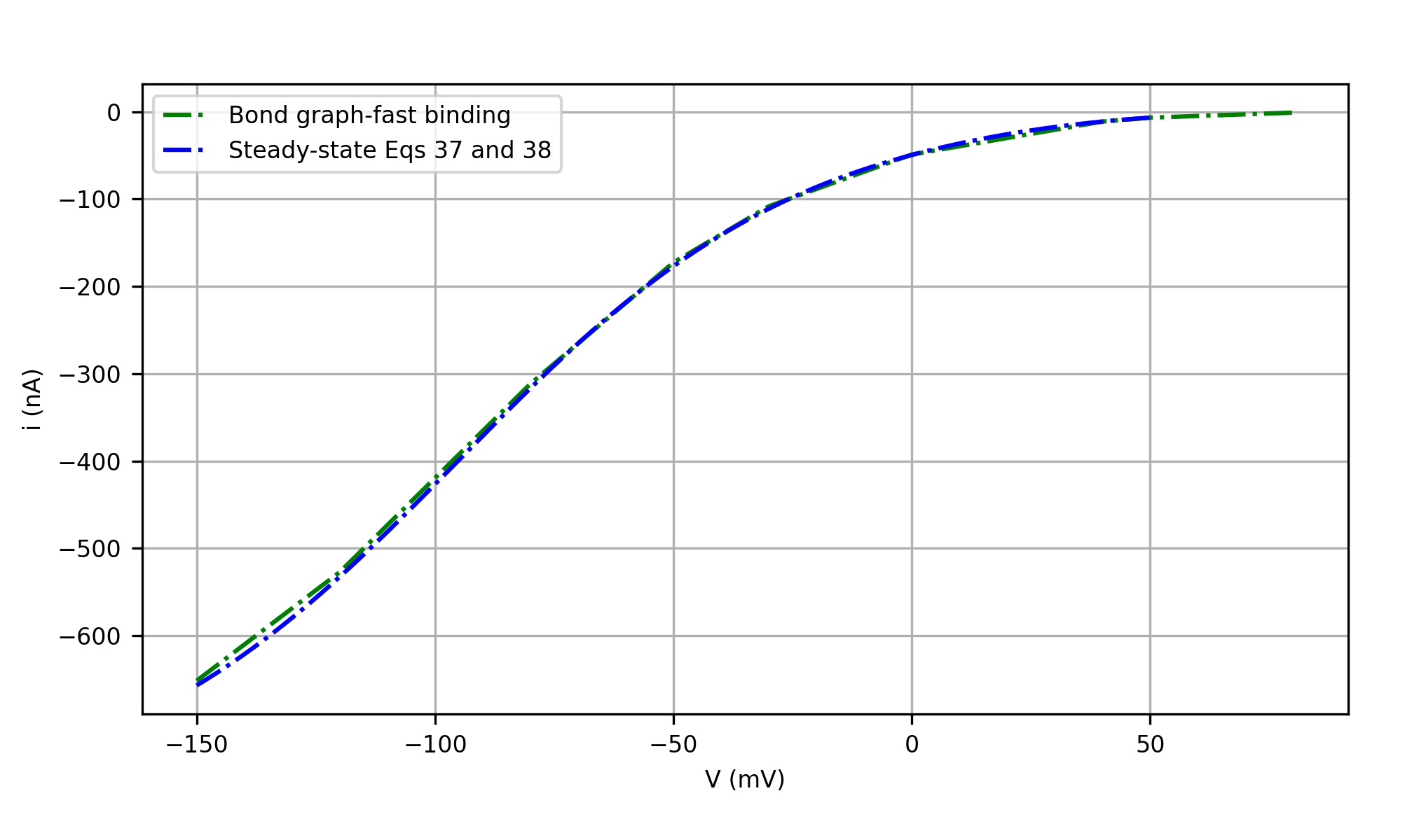
Figure 6:The steady-state results predicted by the full bond graph model, compared with the results from the reduced steady-state model. Both simulations use the assumption of fast binding/unbinding. This is Figure 10 in Hunter et al. (2025).
Table 13:The bond graph parameters for SLC5A1 with the fast binding/unbinding assumption.
[head=false, tabular=ccc, table head=, late after line=
, late after first line=
, table foot=, ]SGLT1_BG_fast.csv & &
Figure 6 shows the steady-state fluxes from the bond graph model (encoded in SGLT1_BG_fast.cellml) and steady-state models (encoded in SGLT1_ss_fast.cellml) using the parameters in Table 13, which confirms that the analytic steady-state equations 37 and 38 is a good approximation of the full bond graph model when the fast binding and unbinding assumption holds, and the slippage (reaction in Figure 4 ) is negligible.
To get the steady state flux from the full bond graph </Electrogenic cotransporter/SGLT1_BG_fast.cellml>, we need to use OpenCOR to manually run each simulation and export the required output variables. The SED-ML file </Electrogenic cotransporter/SGLT1_BG_fast.sedml> provides the required simulation settings. For each simulation, the readers need to modify the test potential (variable test_volt in the component run_SGLT1_BG) to one of the values -0.15, -0.12, -0.08, -0.05, -0.03, 0, 0.04, 0.05, 0.08 (), and the extracellular glucose concentration (variable Glco in the component run_SGLT1_BG) to () or 1 () for before and after addition of glucose, respectively.
The variables to export are V0_Vm and Ii in the component SGLT1_BG. For the Python script mergeData_SGLT1.py in the src folder to process the data, readers must export the simulation data as a CSV file and follow a specific format when naming these files. The string indicating the experiment is SGLT1_BG_step_ss_fast_Data, followed by the glucose condition and the test potential in .
For example, SGLT1_BG_step_ss_fast_Data_sugar_m50mV.csv denotes the test potential is -50 () and extracellular glucose concentration is 1 (), while SGLT1_BG_step_ss_fast_Data_50mV.csv indicates the test potential is 50 () and extracellular glucose concentration is () (no sugar present in the filename). Under default conditions, the Ii value should be approximately 5,658,461.44 at the end of the simulation, while Ii equals 399,880.12 when test_volt is set to 0 V. Please note that the value may vary slightly due to numerical solving errors on different computers.
We have provided the data in <Electrogenic cotransporter\ CellMLV2\ sim_results>. The simulation protocol and the calculation process for the I-V curve are the same as for Fig. 5 in Parent et al. (1992), which will be detailed in the following section.
4.2Simulation results
We followed the experiment conditions in Parent et al. (1992) to simulate the time course of the carrier-mediated currents (Fig.10 in Parent et al. (1992)) and the steady-state glucose-dependent I-V curve (Fig.5 in Parent et al. (1992)). The experiment conditions for Fig. 5 and Fig. 10 in Parent et al. (1992) are summarized in Table 14.
Table 14:The experiment conditions in Fig.5 and Fig. 10 of Parent et al. (1992).
| p1.4cm|X|c|c|p2cm|p3cm Variable | Meaning | Value | Unit | Fig # | Remark |
| intracellular concentration | 20 | Fig.5, Fig.10 | |||
| extracellular concentration | 100 | Fig.5, Fig.10 | |||
| intracellular glucose concentration | 10e-3 | Fig.5, Fig.10 | |||
| extracellular glucose concentration | 0 | Fig.5, Fig.10 without glucose | |||
| extracellular glucose concentration | 1 | Fig.5, Fig.10 with glucose | |||
| the number of transporters per oocyte | Fig.5, Fig.10 | ||||
| Holding potential | -50 | Fig.5, Fig.10 | |||
| Test potential | 50 and -150 | Fig.10 | More values for Fig. 5. |
We use the parameters in Table 11 with the experiment conditions specified in Table 14 to simulate the time course of the carrier-mediated currents of the bond graph model as shown in Figure 7.
![The time course of the carrier-mediated currents. (a) The electrical current when [Glc]_o=0 (mM), and (b) the current when [Glc]_o=1 (mM); The output of the bond graph model is the current -I_i, and the data of were derived using digitizing software Engauge from Fig 10 . This is Figure 11 in .](https://pub.curvenote.com/019992e3-2ea5-72a7-85c1-3c73ef224b6b/public/SGLT1_fit_fig10-0790606f71975c43db7c099ac3a95313.png)
Figure 7:The time course of the carrier-mediated currents. (a) The electrical current when (), and (b) the current when (); The output of the bond graph model is the current , and the data of Parent et al. (1992) were derived using digitizing software Engauge Mitchell et al., 2020 from Fig 10 Parent et al., 1992. This is Figure 11 in Hunter et al. (2025).
A pulse protocol is applied. The holding potential is -50 (), and at time (), the potential was stepped to the test potential for 80 () Parent et al., 1992. The test potentials are 50 () and -150 () for upper plots and lower plots in Fig 10 Parent et al., 1992, respectively. For the bond graph model, we applied the test potential at () to allow the system to reach steady-state. In Figure 7, we aligned the simulation traces with the data from Parent et al. (1992).
In the bond graph model (encoded in SGLT1_BG.cellml), the positive sign of with indicates the current from extracellular to intracellular, while the direction of current in Parent et al. (1992) is from intracellular to extracellular. Hence, we show the model currents before and after the addition of glucose in Figure 7.
To produce the steady-state glucose-dependent I-V curve in Fig 5 Parent et al., 1992, we apply a range of test potentials including -150, -120, -80, -50, -30, 0, 40, 50, 80 () and the parameters in Table 12. After the application of test potential at (), the current at () is saved as steady-state value. For each test potential, we simulated the steady-state current under two conditions: before and after the addition of glucose (i.e., when () and ()). The glucose-dependent current was calculated using the difference in the current values when () and (). The bond graph simulated result is shown in red plot in Figure 8. The data from Parent et al. (1992) were derived using digitizing software Engauge Mitchell et al., 2020.
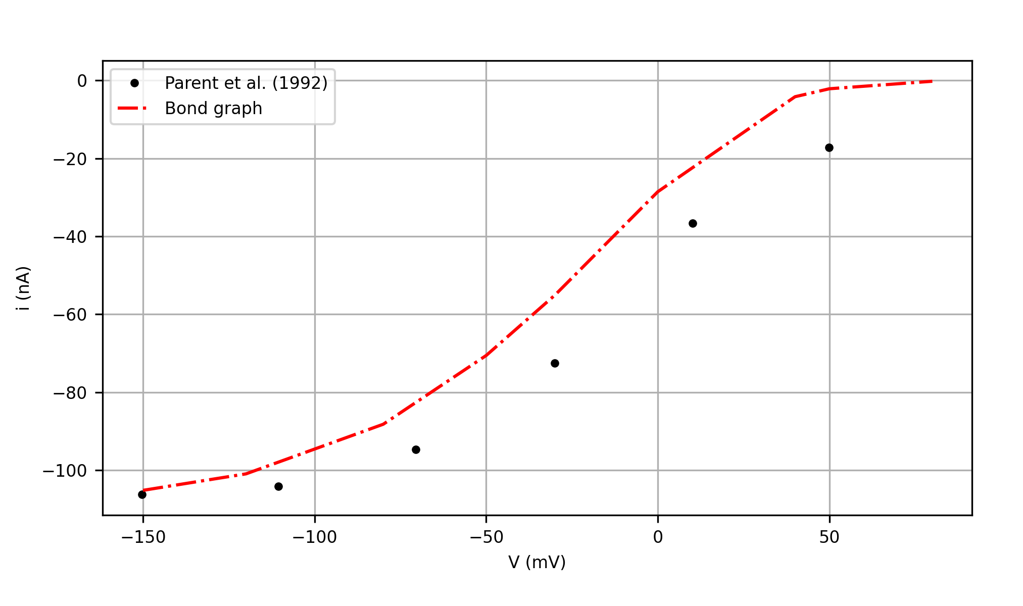
Figure 8:The steady-state glucose-dependent I-V curve of the full bond graph model compared with the data in Fig. 5 in Parent et al. (1992). This is Figure 12 in Hunter et al. (2025).
We have provided the Python scripts under the folder <src> to run the simulations and plot the data, while the SED-ML files in <Electrogenic cotransporter\ CellMLV2> detail the simulation settings. To get the result in Figures 8 and 7, the Python scripts sim_SGLT1.py, mergeData_SGLT1.py, plot_SGLT1.py should run in sequence.
5Conclusion
We have provided here detailed information on the two exemplar models presented in Hunter et al. (2025) to demonstrate the application of the energy-based modelling framework. The derivation of the bond graph parameters has been shown and instructions on reproducing the simulation experiments presented in Hunter et al. (2025) provided. All the required model definition files and execution scripts are provided in the OMEX archive associated with this article.
Not given in Lowe & Walmsley (1986), we use a large number to align with the fast binding assumption Lowe & Walmsley, 1986Hunter et al., 2025.
Apply the constraint ().
Apply the constraint ()
is calculated by the detailed balance equations .
is calculated by the detailed balance equations .
is calculated by the detailed balance equations .
is calculated by the detailed balance equations .
- Hunter, P. J., Ai, W., & Nickerson, D. P. (2025). Energy-based bond graph models of glucose transport with SLC transporters. Biophysical Journal, 124(2), 316–335. https://doi.org/10.1016/j.bpj.2024.12.006
- Cuellar, A. A., Lloyd, C. M., Nielsen, P. F., Bullivant, D. P., Nickerson, D. P., & Hunter, P. J. (2003). An Overview of CellML 1.1, a Biological Model Description Language. SIMULATION, 79(12), 740–747. 10.1177/0037549703040939
- Yu, T., Lloyd, C. M., Nickerson, D. P., Cooling, M. T., Miller, A. K., Garny, A., Terkildsen, J. R., Lawson, J., Britten, R. D., Hunter, P. J., & Nielsen, P. M. F. (2011). The Physiome Model Repository 2. Bioinformatics, 27(5), 743–744. 10.1093/bioinformatics/btq723
- Lowe, A. G., & Walmsley, A. R. (1986). The kinetics of glucose transport in human red blood cells. Biochimica et Biophysica Acta (BBA)-Biomembranes, 857(2), 146–154.
- Pan, M. (2019). A bond graph approach to integrative biophysical modelling. [Phdthesis]. University of Melbourne, Parkville, Victoria, Australia.
- McLaren, C. E., Brittenham, G. M., & Hasselblad, V. (1987). Statistical and graphical evaluation of erythrocyte volume distributions. American Journal of Physiology-Heart and Circulatory Physiology, 252(4), H857–H866.
- Parent, L., Supplisson, S., Loo, D. D., & Wright, E. M. (1992). Electrogenic properties of the cloned Na+/glucose cotransporter: II. A transport model under nonrapid equilibrium conditions. The Journal of Membrane Biology, 125, 63–79.
- Eskandari, S., Wright, E., & Loo, D. (2005). Kinetics of the reverse mode of the Na+/glucose cotransporter. The Journal of Membrane Biology, 204, 23–32.
- Mitchell, M., Muftakhidinov, B., Winchen, T., Wilms, A., Schaik, B. van, badshah400, Mo-Gul, Badger, T. G., Jędrzejewski-Szmek, Z., kensington, & kylesower. (2020). markummitchell/engauge-digitizer: Nonrelease. Zenodo. 10.5281/zenodo.3941227