A theoretical model of slow wave regulation using voltage-dependent synthesis of inositol 1, 4, 5-trisphosphate
Abstract
The system of equations and figures presented in Imtiaz et al. (2002) are verified and reproduced in the current curation paper. Here, to demonstrate reproducibility, We describe the model encoded in the CellML and document the differences between our curated model and the one published by Imtiaz et al. (2002). From the primary publication, we extracted data applying the Engauge digitizer software Mitchell et al., 2020 to compare the current CellML simulation results against those in the primary publication.
1Introduction
Slow waves are rhythmic bioelectrical depolarizations that initiate and control the mechanical activity of gastrointestinal (GI) smooth muscles. One of the mechanisms responsible for generating slow waves involves IP-induced calcium release and calcium-induced calcium release from IP-operated intracellular calcium stores. The resultant calcium increases in the subplasmalemmal space then activate calcium-sensitive inward currents across the plasmalemma that result in slow-wave depolarizations Dicker et al., 2018Imtiaz et al., 2002.
According to Imtiaz et al. (2002), IP oscillations are unnecessary for calcium oscillations, as IP oscillations can occur in many different cell types. In the current work Imtiaz et al. (2002), the authors are introducing a new feedback mechanism based on membrane potential, which then modulates IP synthesis. Where the aim is to study the role of membrane potential feedback on IP synthesis and its role in regulating calcium release and slow waves. The system is simplified by considering a single isopotential cell with a single IP receptor-operated intracellular calcium pool. The ryanodine receptor is ignored in the model. It is important to note that the voltage-dependent channels are considered to be blocked.
A persistent workspace for this work is available in the Physiome Model Repository at https://
This implementation includes the Python source code to generate the model simulations in a ’Simulations’ directory. The corresponding CellML implementation is available in a ’Experiments’ directory containing the encoded mathematical model. This CellML file does not reproduce the figures due to limited solver capabilities at the time of testing. As such, we have elected to describe the required simulation experiments in Python and use the OpenCOR Garny & Hunter, 2015 Python interpreter to perform the simulations and analyses. In this manuscript, we focus on reproducibility and reusability.
2Model description
2.1Primary Publication
The model was formulated using a Hodgkin-Huxley type formulation. The cell membrane lipid bilayer was modelled as a capacitance (C), and the ion channels in the membrane were represented as conductance. The change in the transmembrane potential (V) over time depended on the sum of the individual ion currents in the cell:
2.2Model Implementation
The implementation of the model was performed using CellML Cuellar et al., 2003. Some simulation values stated in Imtiaz et al. (2002) resulted in different model behaviour, which we adjusted as outlined in Table 1. The simulation experiments presented here were performed using OpenCOR (Snapshot 2021-10-5 Garny & Hunter, 2015). Simulation settings and detailed solver information were encoded in SED-ML ducument Waltemath et al., 2011.
We reproduced the data represented in Imtiaz et al. (2002, Figures 2A, 3A, 4A, 6(A and B) & 8A) by using different settings corresponding to the various model experiments. We implemented the model configuration in Python scrip for each experiment. Then, we perform the Python script to plot the related data.
The name of the simulation and plot scripts indicates the figure number in the primary paper. For example, Fig2_sim.py is used to generate the simulation data, and Plot_Fig2.py reproduces the graph shown in Figure 2A from Imtiaz et al., 2002.
2.3Model Modifications 
Mathematical Equations were the same as reported in the primary publication of Imtiaz et al. (2002) except for Imtiaz et al. (2002, Equations 3, 7, and 9). Please see the correction in below:
Unit consistency:
In Eq. 7, the first term, which indicates the lump current () should carry a negative sign, while in the original work, the lump current is presented with a positive sign.
In Eq. 7, we correct the consistency in time unit by multiplying the denominator on the right-hand side by the scale factor of 60 s
In Eq. 9, the term indicates the external stimuli has a unit of while the term which indicates IP concentration in the cytosol has a unit of . The baseline parameter values are provided in the primary paper Imtiaz et al. (2002).
Table 1:Correction of primary Imtiaz et al. (2002, Tables 1,2 & 3)
Table Parameter Primary paper CellML Table 1 Table 3
No initial condition was defined in the primary paper, all initial conditions extracted from the original paper, using Engauge Digitizer software Mitchell et al., 2020.
Table 2:Initial conditions on the current CellML implementations.
-65.00 4.113 0.478 0.408 0.7533 In the case of model experiments and simulations, there was no clear information about the protocol details they used to inject the current (stimulus) into the cell. The simulation experiments we have inferred from the primary paper in order to reproduce the simulation results are described in Section 2.4.
2.4Model Simulations
In the presented figures, the dots denote the simulated data extracted from the primary publication, while the solid lines are the simulation results produced by the current CellML implementation.
Figure 3A was reproduced applying the following protocols (2), while the initial conditions were the same as Table 2.
Figure 4A was reproduced using the IP model by setting the initial membrane potential (V) at a fixed holding potential -65.09 mV and then polarizing the membrane by injecting the current into the cell, for more details information see (3) and Figure 3.
In Figure 8A, the effect of the interpulse duration on current pulse-induced responses was studied. The aim was to demonstrate the pulse would fail to evoke responses if the interpulse duration was reduced below a critical value. In Fig 8A , while in Fig 8B .
2.5Model Results
We employed Engauge Digitizer software Mitchell et al., 2020 to extract data from all figures from Imtiaz et al. (2002) to present alongside the results of the present work. The reproduction of all figures of Imtiaz et al. (2002) is given in Figures 1-5, which show good agreement with the data of the primary paper. Solid lines show the output from the current curation, and crosses show discrete points found by the Engauge Digitizer of the figures originally published article.
Applying some corrections to the original equations and parameters (see model modifications), the following results were produced:
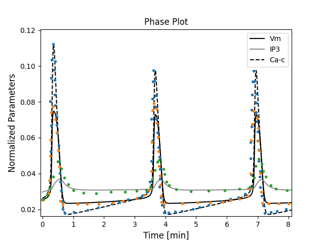
Figure 1:The primary data (*) of Imtiaz et al. (2002, Figure 2A) with our reproduction of all subfigures. To reproduce Imtiaz et al. (2002, Figure 2A), use the Python manuscript Fig2_sim.py and to plot it use Plot_Fig2.py.
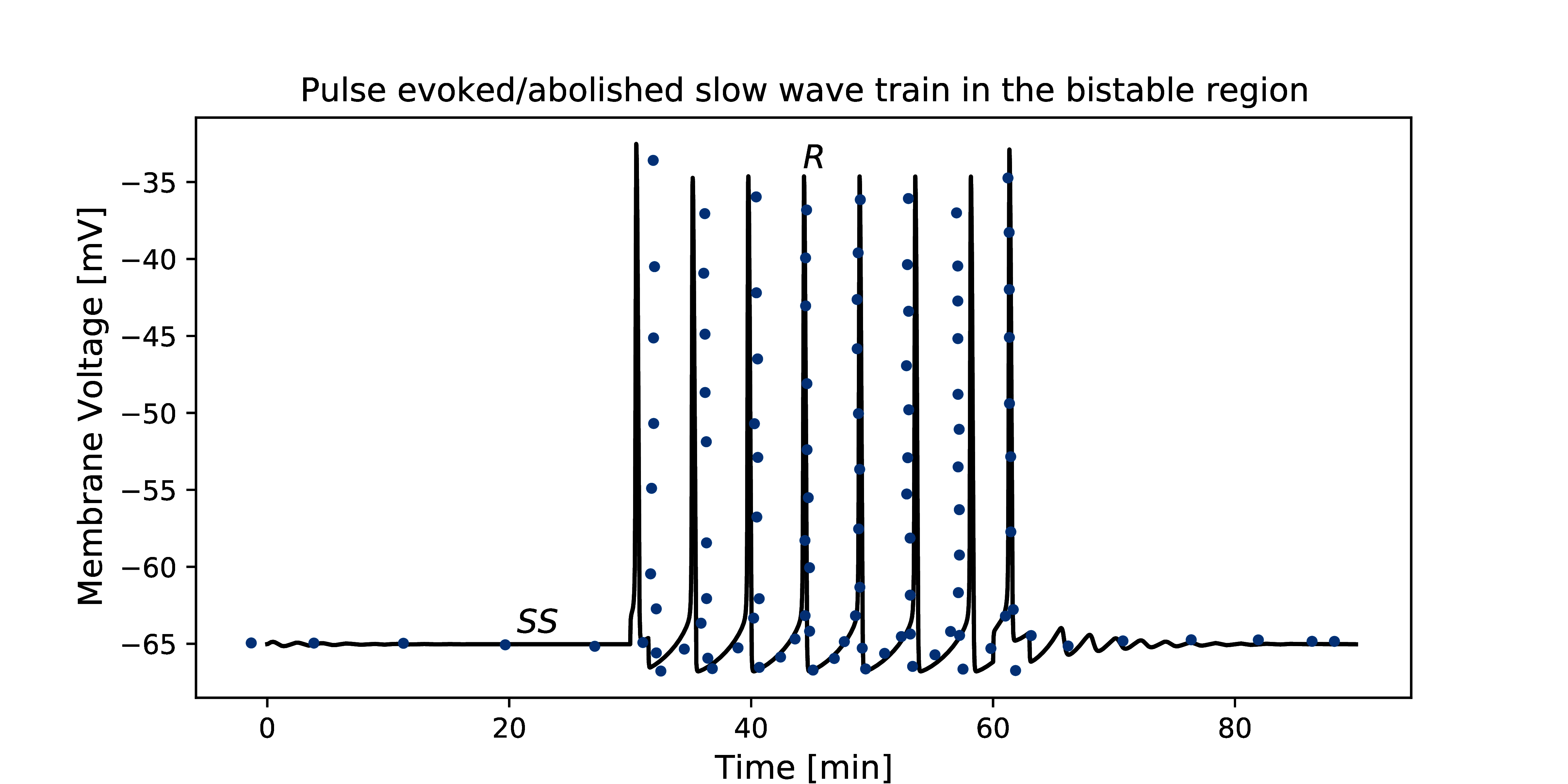
Figure 2:The primary data (*) of Imtiaz et al. (2002, Figure 3A) with our reproduction of all subfigures. To reproduce Imtiaz et al. (2002, Figure 3A), use the Python script Fig3_sim.py and to plot it use Plot_Fig3.py.
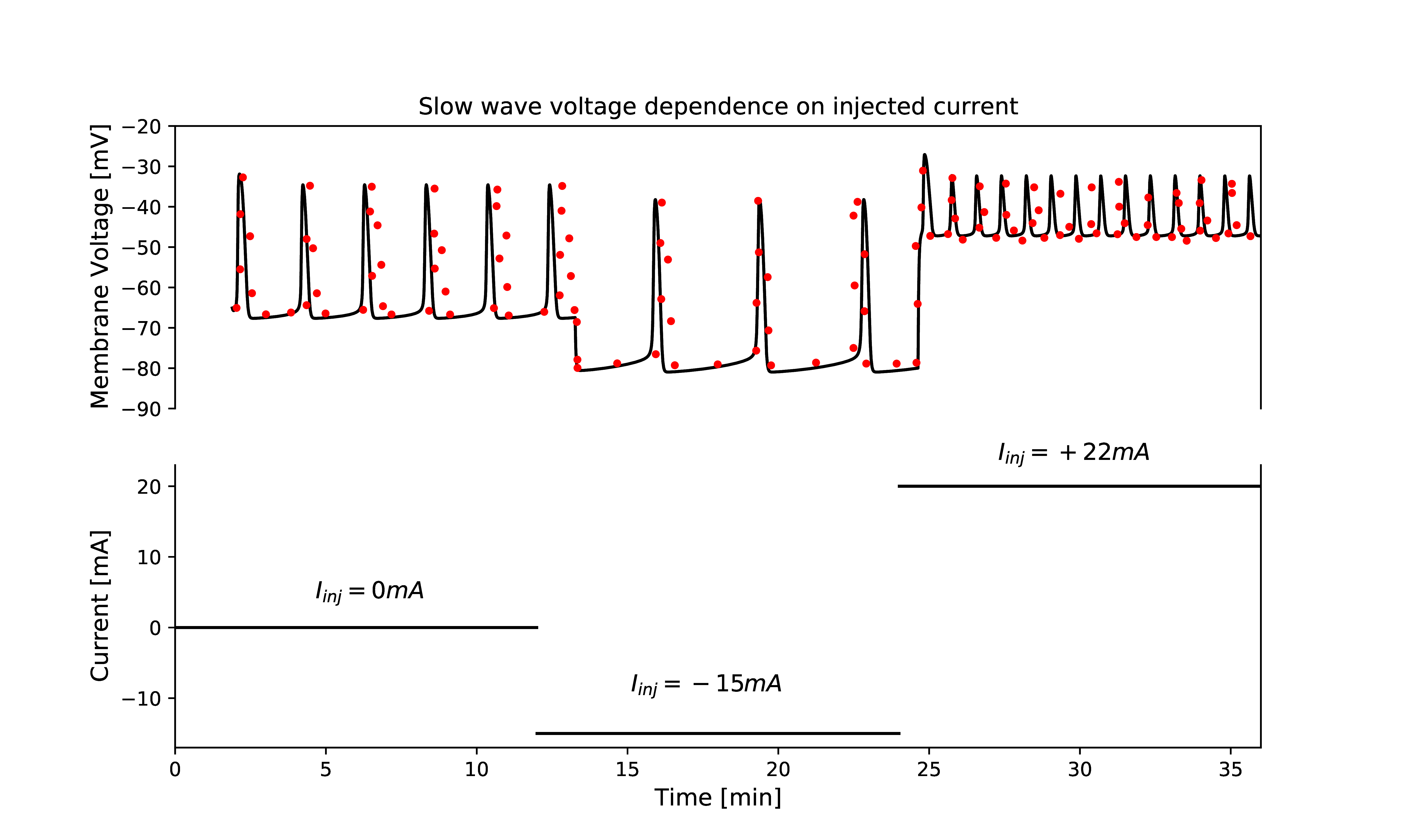
Figure 3:The primary data (*) of Imtiaz et al. (2002, Figure 4A) with our reproduction of all subfigures. To reproduce Imtiaz et al. (2002, Figure 4A), use the Python script Fig4_sim.py and to plot it use Plot_Fig4.py.
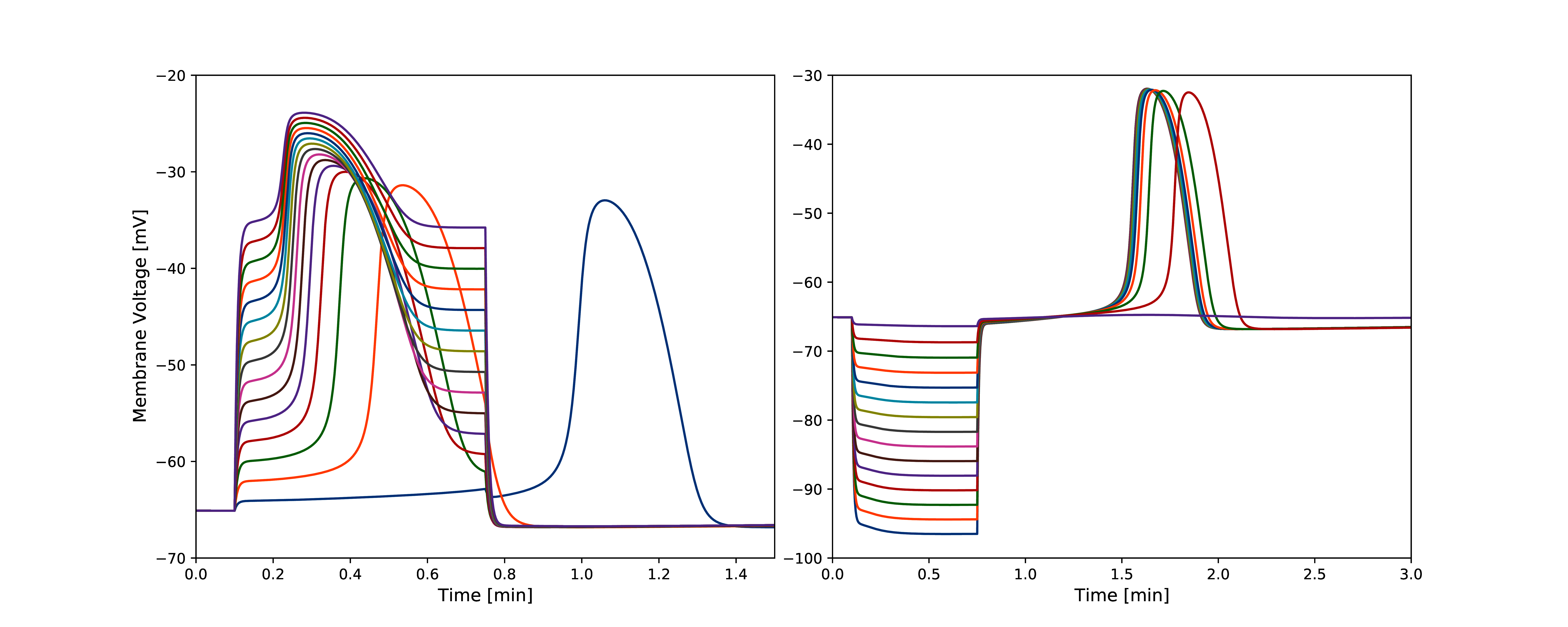
Figure 4:The primary data (*) of Imtiaz et al. (2002, Figure 6(A and B)) with our reproduction of all subfigures. To reproduce Imtiaz et al. (2002, Figure 6(A and B)), use the Python script Fig6_sim.py and to plot it use Plot_Fig6.py.
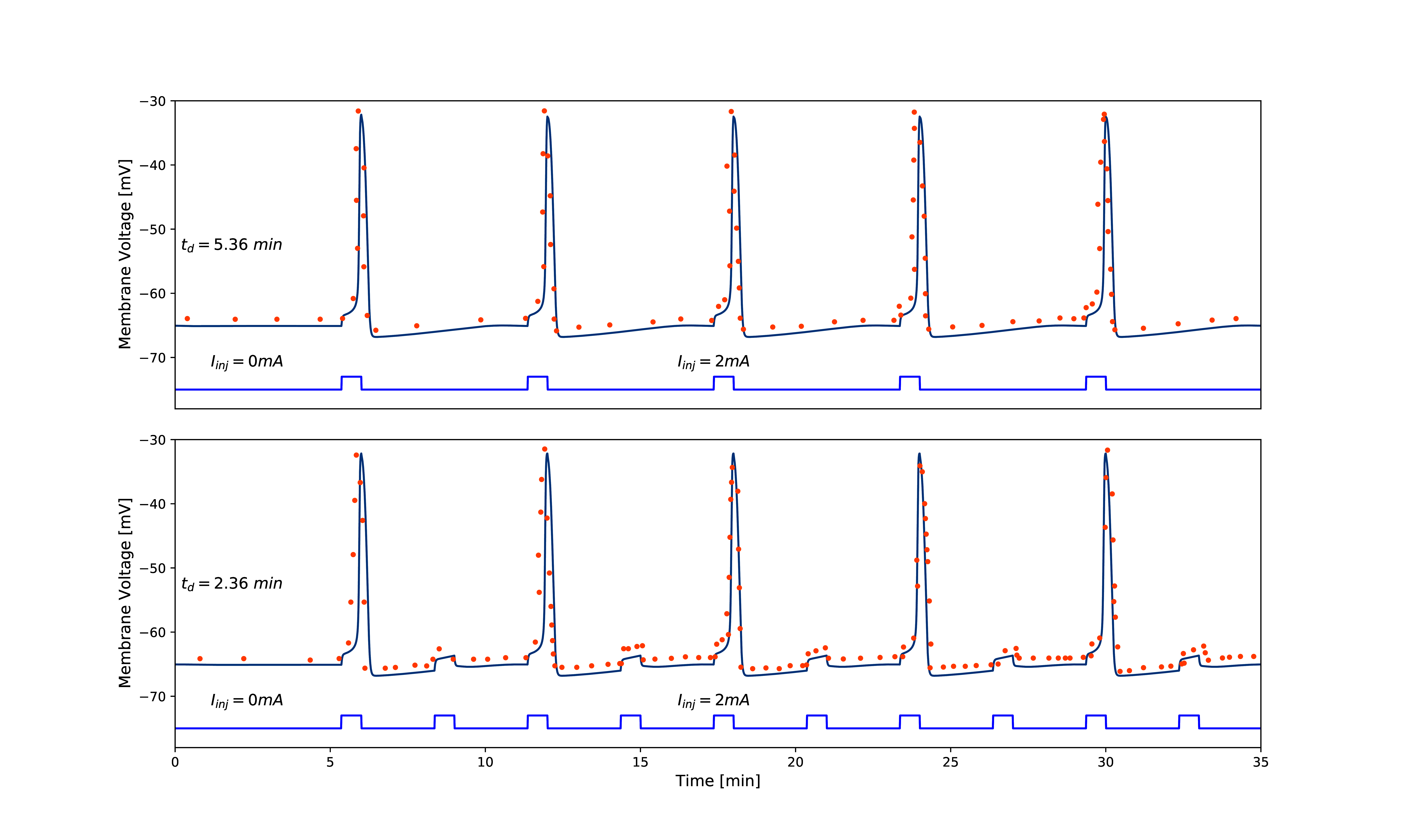
Figure 5:The primary data (*) of Imtiaz et al. (2002, Figure 8A) with our reproduction of all subfigures. To reproduce Imtiaz et al. (2002, Figure 8A), use the Python script Fig8_sim.py and to plot it use Plot_Fig8.py.
3Discussion
We implemented the model of Imtiaz et al. (2002) using CellML which can be reused in future. We successfully replicated simulation results and summarized detailed experiment settings for simulation in Section 2.4. In doing this, we noticed trivial typographical errors in parameter units and references in Imtiaz et al. (2002, Table 1, 3). Hence, we highlighted the issues and added correction to remove potential confusion in Section 2.3.
Acknowledgments
The authors gratefully acknowledge the support of the Ministry of Business, Innovation and Employment’s Catalyst Strategic Fund (12 Labours).
- Imtiaz, M. S., Smith, D. W., & van Helden, D. F. (2002). A theoretical model of slow wave regulation using voltage-dependent synthesis of inositol 1, 4, 5-trisphosphate. Biophysical Journal, 83(4), 1877–1890. 10.1016/S0006-3495(02)73952-0
- Mitchell, M., Muftakhidinov, B., Winchen, T., Wilms, A., van Schaik, B., badshah400, Mo-Gul, Badger, T. G., Jędrzejewski-Szmek, Z., kensington, & kylesower. (2020). markummitchell/engauge-digitizer: Nonrelease. 10.5281/zenodo.3941227
- Dicker, D., Nguyen, G., Abate, D., Abate, K. H., Abay, S. M., Abbafati, C., Abbasi, N., Abbastabar, H., Abd-Allah, F., Abdela, J., & others. (2018). Global, regional, and national age-sex-specific mortality and life expectancy, 1950–2017: a systematic analysis for the Global Burden of Disease Study 2017. The Lancet, 392(10159), 1684–1735.
- Bergmann, F. T., Adams, R., Moodie, S., Cooper, J., Glont, M., Golebiewski, M., Hucka, M., Laibe, C., Miller, A. K., Nickerson, D. P., Olivier, B. G., Rodriguez, N., Sauro, H. M., Scharm, M., Soiland-Reyes, S., Waltemath, D., Yvon, F., & Novère, N. L. (2014). COMBINE archive and OMEX format: one file to share all information to reproduce a modeling project. BMC Bioinformatics, 15(1), 369. 10.1186/s12859-014-0369-z
- Garny, A., & Hunter, P. J. (2015). OpenCOR: a modular and interoperable approach to computational biology. Computational Physiology and Medicine, 6, 26. 10.3389/fphys.2015.00026
- Cuellar, A. A., Lloyd, C. M., Nielsen, P. F., Bullivant, D. P., Nickerson, D. P., & Hunter, P. J. (2003). An Overview of CellML 1.1, a Biological Model Description Language. SIMULATION, 79(12), 740–747. 10.1177/0037549703040939
- Waltemath, D., Adams, R., Bergmann, F. T., Hucka, M., Kolpakov, F., Miller, A. K., Moraru, I. I., Nickerson, D., Sahle, S., Snoep, J. L., & others. (2011). Reproducible computational biology experiments with SED-ML-the simulation experiment description markup language. BMC Systems Biology, 5(1), 1–10.


