A kinetic model of β-adrenergic control in cardiac myocytes
Abstract
The system of equations and figures presented in Saucerman et al. (2003) are verified and reproduced in this paper’s curation effort. These checks are performed in MATLAB. With some parameter additions and modifications, we can reproduce all figures with small mismatches.
1Introduction
-adrenergic signalling within the cardiac myocyte is a well-documented signalling pathway, but few mathematical models exist of the complete system. Saucerman et al. (2003) published such a model of the activation of the signalling cascade from a ligand binding the receptor on the cell surface, to triggering the activation of the beta-1 adrenergic receptor (1AR), cyclic AMP (cAMP), adenylyl cyclase (AC), protein kinase A (PKA), and phospholamban (PLB). Subsequent downstream effects on ion channel activity are the result, notably through modifying the activity of calcium channels in the regulation of an action potential.
This present work involves the mathematical curation the model. MATLAB MATLAB, 2017 code was obtained from the first author of Saucerman et al. (2003) in an effort to reproduce the figures of that paper. While there is not an exact correspondence between equations presented in the paper and code provided, the figure trends are still reproduced, and numeric values are matched with some modifications/additions made to parameter values, as detailed in under Model Modifications.
A persistent workspace of the code is available in the Physiome Model Repository, at https://
This workspace includes the MATLAB source code for running the model. The corresponding CellML Cuellar et al., 2003 implementation is available at https://
2Model description
The model is broken into several modules:
1AR activation
Gs protein activation
cAMP metabolism
PKA activation
PLB regulation
L-type calcium channel (LCC) regulation
Once the cell is activated by an agonist isoproterenol (Iso), the collective effects of these modules are studied downstream. This includes changes to ion channel activity towards the production and management of an action potential.
3Model Modifications
3.1Mathematical Equations
These are the same as reported in the supplementary material of Saucerman et al. (2003) with the exception of the L-type calcium channel. This is a reduced-state version of the original model by Jafri et al. (1998), which was implemented in the MATLAB code provided by the original author. The version of the model published in Saucerman et al. (2003) showed a complete version of the model as in Jafri et al. (1998), replicated to represent phosphorylated states.
3.2Parameter Values
The baseline parameter values are provided in the supplementary material of Saucerman et al. (2003) and in the MATLAB code provided by Saucerman. Missing values on cell geometry are provided in Table 1 which are used in all Figure reproductions.
| Name | Value | Source |
|---|---|---|
| Myocyte volume | Bers (2001) | |
| Myocyte density | Mendez et al. (1960) |
Table 1:Parameters sourced for the model, which were not included in the primary paper.
It was found that the density of myocytes needed to increase by 6.4 times in order to better match the primary paper figures.
| Figure | Parameter values | Number of iterations | T (min) |
|---|---|---|---|
| 2a | 1 | 18 | |
| 2b | 6 | ||
| 8 | |||
| 2c, 2d | 6 | 1 | |
| 2e | 20 | 30 | |
| 2f | 2 | 1 | |
| 2g, 2h | 2 | 1 | |
| 3a | 32 | 7 | |
| 3b | 32 | 7 | |
| 4a, 4b | 3 | 3 | |
| 5 | 24 | 20 | |
| 6a | 3 | 1 | |
| 6b | 4 | 1 | |
| fracPLB | |||
| fracPLBo |
Table 2:Specific protocol followed in the reproduction of each figure, run for a span of T minutes. indicate multiplication or division of parameter by the specified value respectively. denotes the variable value being changed with every iteration. One iteration constitutes running the entire model once. For multiple species being changed for one figure: for the th loop iteration, the value of the species is given by the th value in the sequence given in the sequence (Column 2) for all marked species. (3a, 3b): four separate iterations for every [Iso]: one control, one with changed only, one with changed only, and one with change only. (5): three separate iterations for every [Iso]: one control, one with changed only, one with changed only. patch clamping: Figures 2g-h, 6b follow Protocol 1; Figure 2f follows Protocol 2 (see Table 3).
See primary paper or source code for an explanation of all chemical abbreviations.
Experimental conditions specific to each Figure are given in Table 2. For Figures 2f-h and 6b, patch clamp protocols are defined in Table 3.
This system has 44 dependent variables. Unless stated otherwise, all figure reproductions are subject to the same initial conditions (see source code). These values are embedded in the script main.m.
4Computational Simulation
The system of differential-algebraic equations is solved in MATLAB using stiff solver ode15s Shampine & Reichelt, 1997 with automatic/adaptive time stepping, , . No further packages are required; any machine with the full ODE suite (which includes ode15s solver) should be able to run all simulations.
Run the script main.m. The user will be prompted to specify the desired figure reproduction: input the appropriate string of format where is the figure number and is the subfigure letter: for example, .
Figures are highly recommended to be reproduced using parallel computing (parpool, >=4 workers) in MATLAB due to the size and stiffness of the code. By default, this is already set up in the script. Otherwise, computations will take up to 30 minutes per figure, on a 2.8 Ghz / 4 core machine running on Windows 10. Once running, keep parpool open (change parallel preferences: adjust time to automatically shut down pool after appropriate amount of time) such that time is not lost waiting for the pool to start up on every simulation.
| Figure | Species | Original value | Value modified for MATLAB |
|---|---|---|---|
| 2b | max([Iso]) | ||
| 2c/d | [PKI] | ||
| 2f | Patch clamp voltage | holding , step | holding , step |
| 4a | [IBMX] | ||
| 4b | max([Iso]) | ||
| 5 | PKAI | 0 | 5% of baseline |
| PKI | 0 | 5% of baseline | |
| 6a | [Iso] | - | |
| 6b | [Iso] | - | |
| fracPLB | - | 0 |
Table 4:Modifications made to stated values of primary paper, in the reproduction of the figures.
The original implementation of the model was performed using Berkeley-Madonna software, with a different ODE solver to MATLAB Saucerman et al., 2003. As some simulation values stated in the primary paper resulted in the model being unsolvable in the MATLAB routine, we had to make adjustments as outlined in Table 4.
5Model Results
We employ Engauge Digitizer software Mitchell et al., 2020 to extract data from Figures of Saucerman et al. (2003) to present alongside results of the present work.
![The primary data (x) of Figure 2 with our reproduction of all subfigures (-). Note: (2c) PKA\ activation = \frac{[PKACI]}{2*[PKAI_{tot}]}](https://pub.curvenote.com/f83c8956-ce8c-43c2-afc9-9b638aa131e0/public/F2a-fe967c93c63fabea4181c64f0f2adabd.jpg)
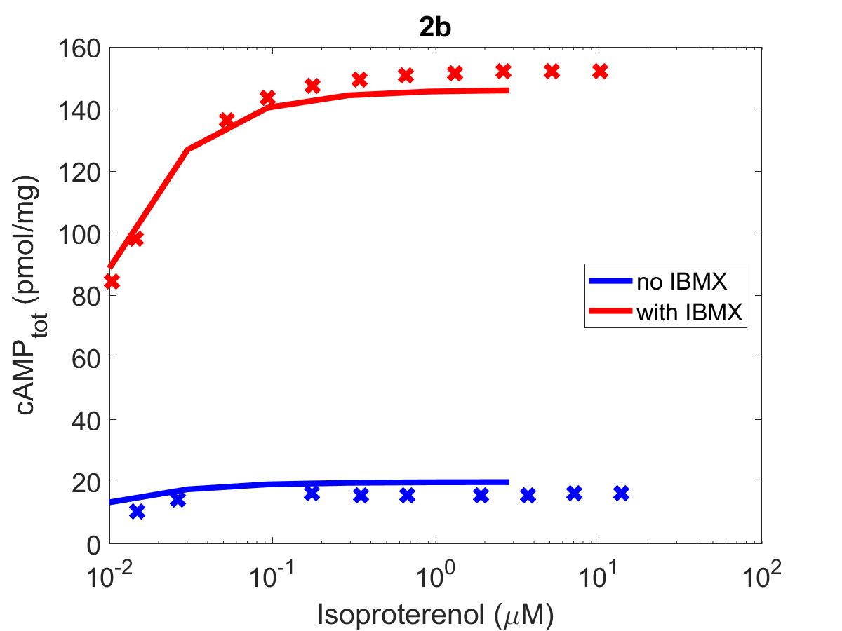

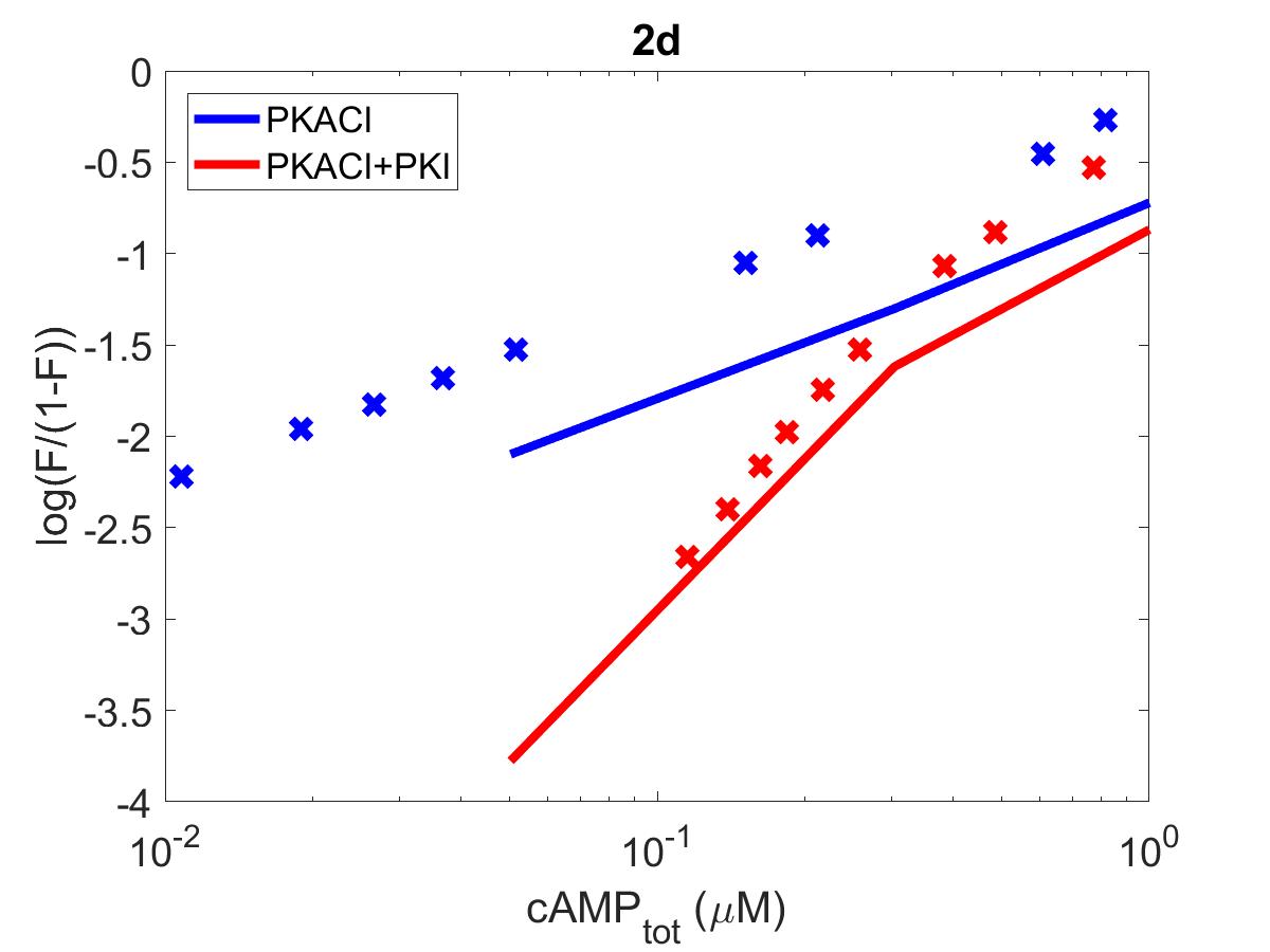
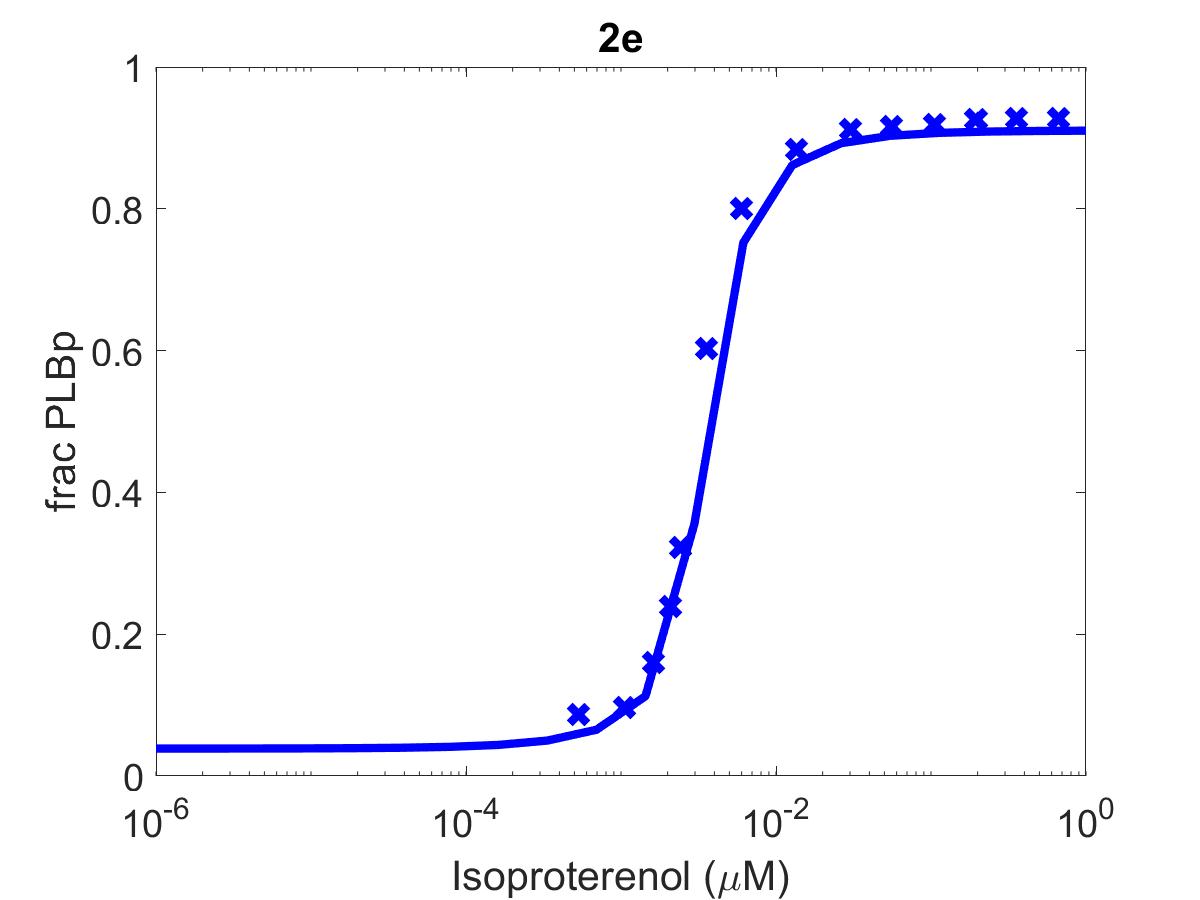
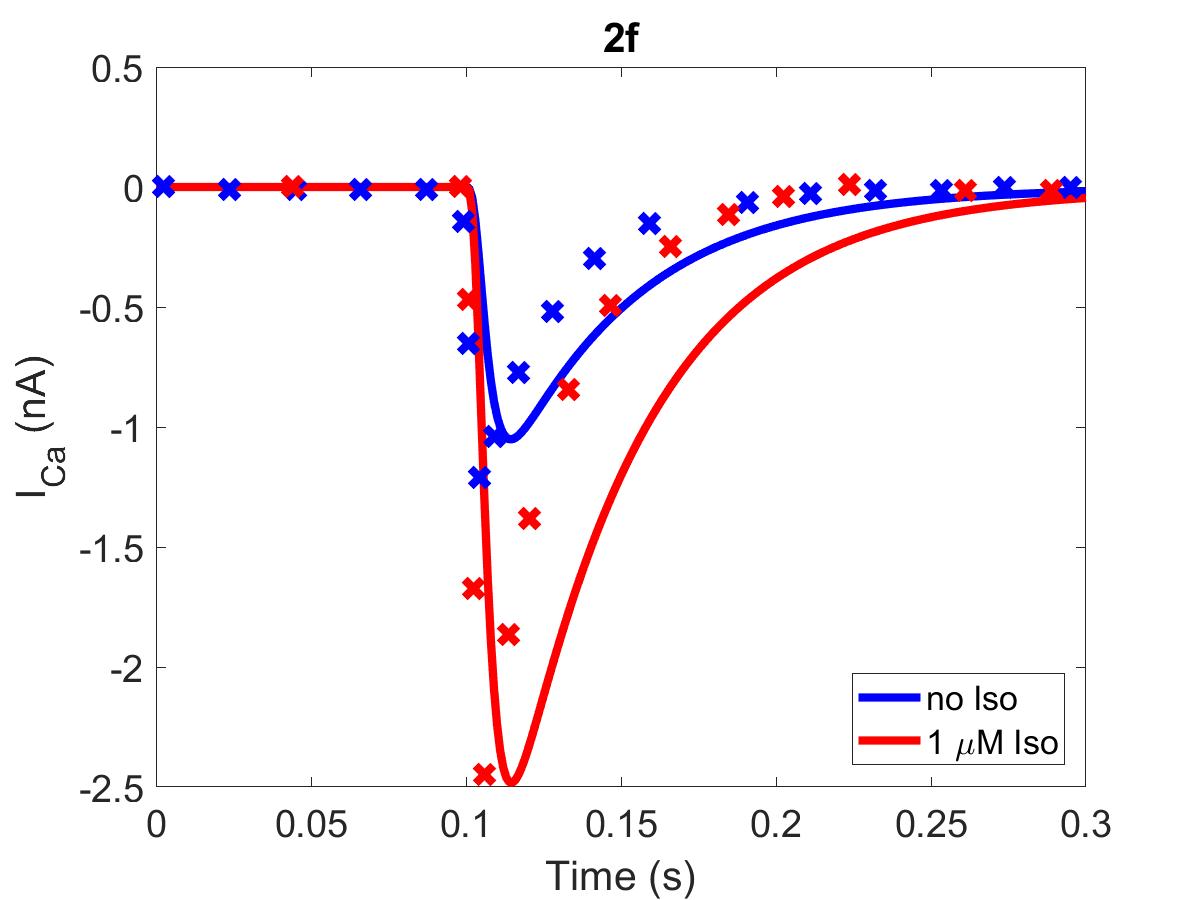
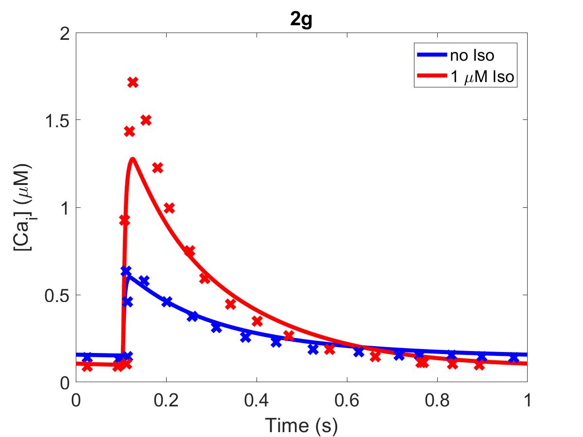
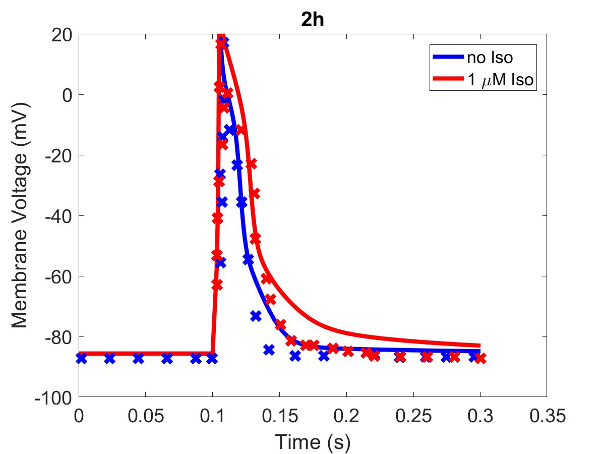
Figure 1:The primary data () of Figure 2 with our reproduction of all subfigures (). Note: (2c)
![The primary data (x) of Figure 3 with our reproduction of all subfigures (-). Note: lines in (3b) showing modifications to [AC]_{tot}, \beta 1AR, K_{Gs\alpha } have been grouped into an average ‘augmentation’ line.](https://pub.curvenote.com/f83c8956-ce8c-43c2-afc9-9b638aa131e0/public/F3a-14d11e23ba474c5ae42f0df8ac88d96d.jpg)
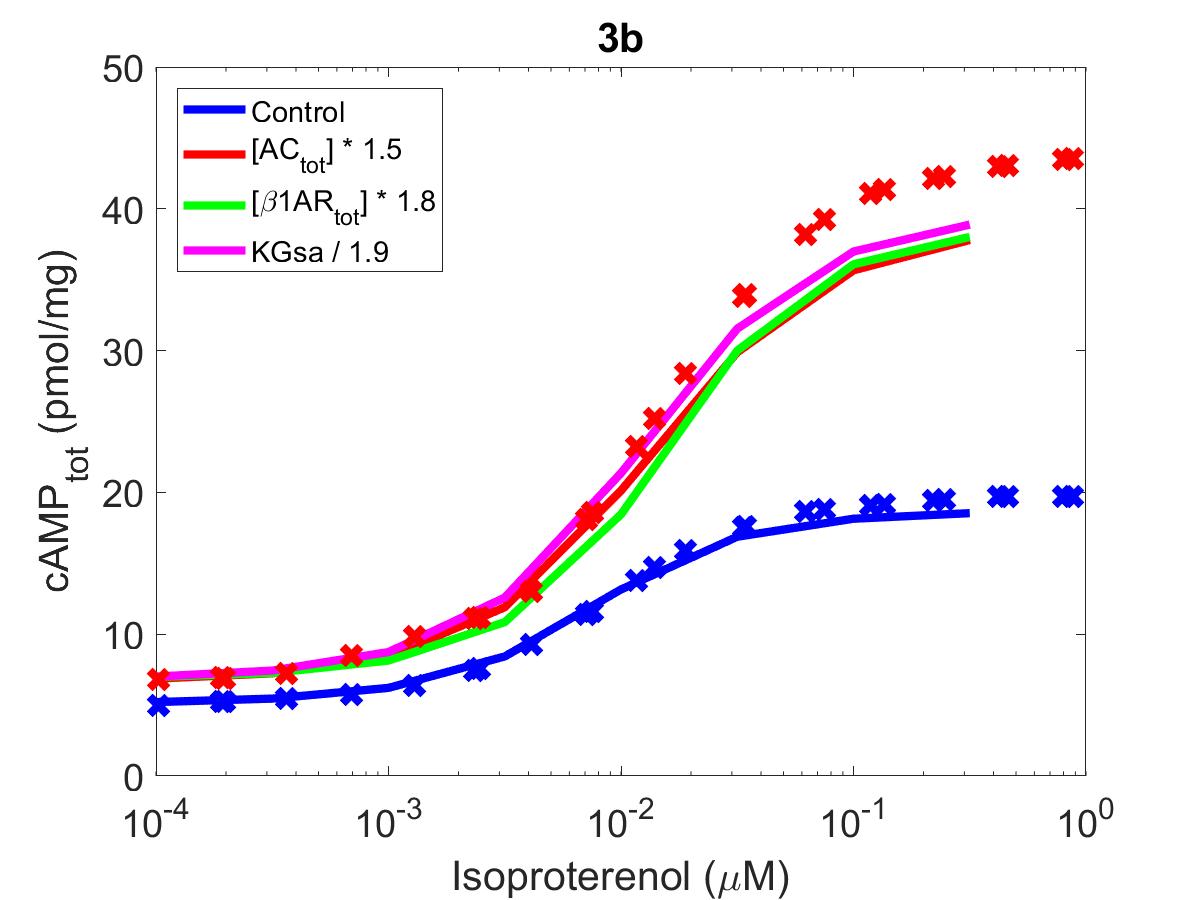
Figure 2:The primary data () of Figure 3 with our reproduction of all subfigures (). Note: lines in (3b) showing modifications to have been grouped into an average ‘augmentation’ line.
![The primary data (x) of Figure 4 with our reproduction of all subfigures (-). (4a): primary data shown in blue, reproduction in red. AC\ activity=cAMP_{tot}. (4b): f_{cAMP}=\frac{cAMP_{tot}}{cAMP_{tot,max}}. Annotated numbers on the graph refer to [Iso] set for that experiment.](https://pub.curvenote.com/f83c8956-ce8c-43c2-afc9-9b638aa131e0/public/F4a-65feb5ffe32f443bd5703639794383d1.jpg)
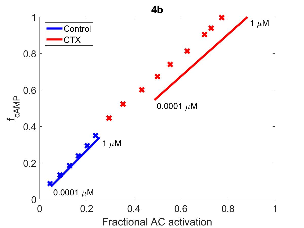
Figure 3:The primary data () of Figure 4 with our reproduction of all subfigures (). (4a): primary data shown in blue, reproduction in red. . (4b): . Annotated numbers on the graph refer to [Iso] set for that experiment.
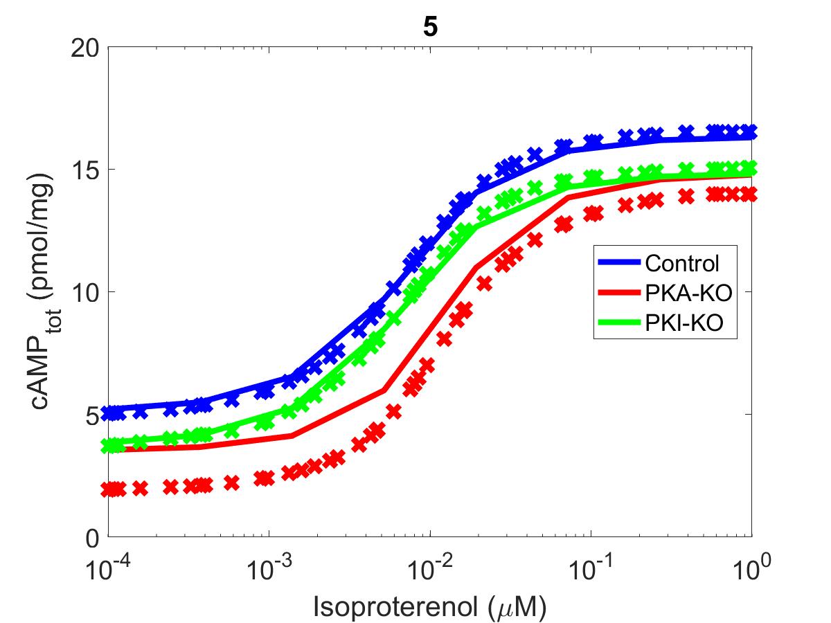
Figure 4:The primary data () of Figure 5 with our reproduction ().
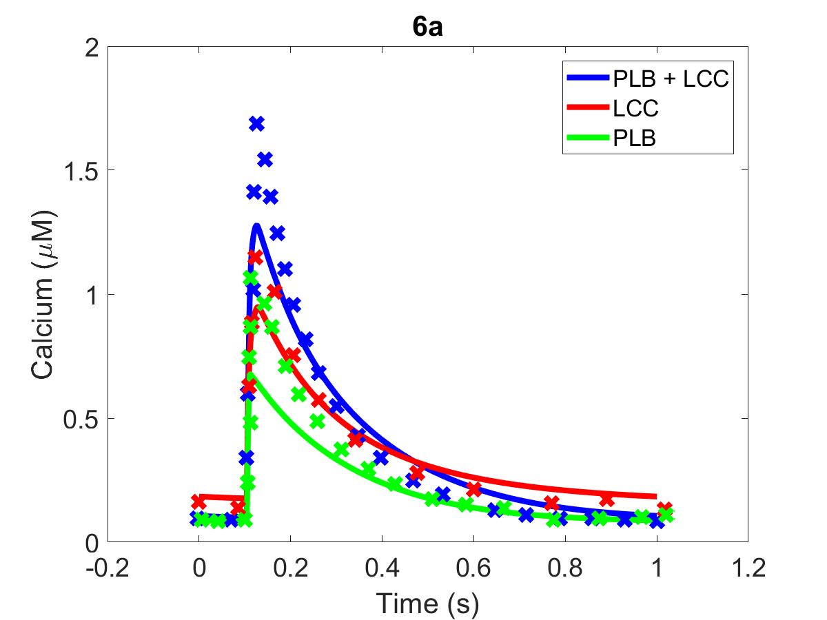

Figure 5:(6a) The primary data () of Figure 6a with our reproduction of all subfigures (). (6b) Primary data shown in blue, reproduction in red.
The reproduction of all figures of Saucerman et al. (2003) are given in Figures 1-5, which show good agreement against the data of the primary paper. Solid lines show the output from this curation effort, and crosses show discrete points found by the Engauge Digitizer of the figures originally published.
6Discussion
We demonstrate that figures of Saucerman et al. (2003) can be reproduced given some additions (Table 1) and adjustments (Table 4) made to model parameter values. There are slight deviations of the curated model output from the original data which can be attributed to parameter modifications we had to make to ensure a simulation runs to completion (see Figures 1c, 1d, 3a, 3b). Other mismatches may be owing to differences from the original implementation in Berkeley-Madonna, which had different solver settings to this effort. The original code is no longer available.
As this paper follows the tenets of FAIR Wilkinson et al., 2016, further credibility is lent to the original model. The model has already proven to be valuable to the mathematical modelling community in understanding the workings of -adrenergic receptor signalling within cardiac myocytes.
- Saucerman, J. J., Brunton, L. L., Michailova, A. P., & McCulloch, A. D. (2003). Modeling β-adrenergic control of cardiac myocyte contractility in silico. Journal of Biological Chemistry, 278(48), 47997–48003.
- MATLAB. (2017). version 9.3.0713579 (R2017b). The MathWorks Inc.
- Cuellar, A. A., Lloyd, C. M., Nielsen, P. F., Bullivant, D. P., Nickerson, D. P., & Hunter, P. J. (2003). An Overview of CellML 1.1, a Biological Model Description Language. SIMULATION, 79(12), 740–747. 10.1177/0037549703040939
- Jafri, M. S., Rice, J. J., & Winslow, R. L. (1998). Cardiac Ca2+ dynamics: the roles of ryanodine receptor adaptation and sarcoplasmic reticulum load. Biophysical Journal, 74(3), 1149–1168.
- Bers, D. (2001). Excitation-contraction coupling and cardiac contractile force (Vol. 237). Springer Science & Business Media.
- Mendez, J., Keys, A., Anderson, J., Grande, F., & others. (1960). Density of fat and bone mineral of the mammalian body. Metabolism, 9, 472–477.
- Shampine, L. F., & Reichelt, M. W. (1997). The matlab ode suite. SIAM Journal on Scientific Computing, 18(1), 1–22.
- Mitchell, M., Muftakhidinov, B., Winchen, T., Wilms, A., van Schaik, B., badshah400, Mo-Gul, Badger, T. G., Jędrzejewski-Szmek, Z., kensington, & kylesower. (2020). markummitchell/engauge-digitizer: Nonrelease (v12.2.1) [Computer software]. Zenodo. 10.5281/zenodo.3941227
- Wilkinson, M. D., Dumontier, M., Aalbersberg, Ij. J., Appleton, G., Axton, M., Baak, A., Blomberg, N., Boiten, J.-W., da Silva Santos, L. B., Bourne, P. E., & others. (2016). The FAIR Guiding Principles for scientific data management and stewardship. Scientific Data, 3(1), 1–9.


